FRB/US with VAR-based Expectations
Getting started
If you wish to run the code of this tutorial, or to experiment for yourself, make sure to follow the instructions in Introduction/Getting_started.
The Model File
We recommend placing the model definition in its own Julia module in a separate source file. Although this is not strictly necessary, it helps to keep the code well organized and it also allows us to take advantage of pre-compilation. The first time we load the model file it takes some time to compile, and after that loading is much faster.
The FRB/US model we will be working with is located in models/FRBUS_VAR.jl. This file was automatically generated from the model.xml file contained within frbus_package.zip.
Some Notes About the Julia Model File
Some variables are declared as log variables using the
@logdeclaration within a@variablesblock. For example@variables model begin # ... # "Investment in equipment, current \$" @log ebfin "Personal consumption expenditures, current \$ (NIPA definition)" @log ecnian # ... # endA full discussion of log variables is beyond the scope of this tutorial. However a very simplified explanation is that this improves the stability of the numerical solver for variables which are always positive.
Variables which do not have an associated equation, and for which data is always given, are declared exogenous using an
@exogenousblock. For example@exogenous model begin # Exogenous variables: "Potential government employment ratio (relative to business)" adjlegrt "Dummy, post-1979 indicator" d79a "Dummy, 1980-1995 indicator" d8095 # ... # endThe EViews syntax is translated to Julia syntax. EViews functions
d()anddlog()are replaced with their equivalent StateSpaceEcon meta functions@d()and@dlog(). EViews@movav()is left alone, because a meta function by the same name already exists in StateSpaceEcon, and does the same thing. Finally, the EViews@recode()is replaced with the equivalent Julia functionifelse(), or where appropriate with amin()or amax().Several equations contain expressions matching the pattern
1 / (1 + exp(-cx)), wherecis a large constant (usually 25) andxis some expression. This sigmoid function is a smooth approximation of the Heaviside step function for large values ofc. While mathematically the derivative of this function is well defined and converges to approximately zero everywhere outside a very small interval containing 0, numerically it causes problems because it results in either 0/0 or ∞/∞. To remedy this situation, we replace such patterns with equivalent calls toheaviside(cx), where the functionheaviside()is defined in the model file.export heaviside "Heaviside step function" @inline heaviside(x) = convert(typeof(x), x>zero(x))
Regenerating the Model File
We have included the script update_models.jl. It is not necessary for running the code below, but it may be helpful for further experimentation.
If the model file is missing, for some reason or another, this script will automatically download frbus_package.zip and process the model.xml within it to re-generate model/FRBUS_VAR.jl. This could also be useful if you make modifications to model.xml (including not only the equations, but also the parameter values), or if you want to use a different FRBUS package from the one posted on the FRBUS website. In this case, simply place your frbus_package.zip in the models/ directory and run update_models.jl. Of course such modifications can also be done directly into the existing models/FRBUS_VAR.jl file.
Note that after updating models/FRBUS_VAR.jl, it'd be best to restart the REPL. The first time you load the new model module it'll take a bit longer due to pre-compilation.
Load the Model
Assuming that the models/ directory is already in the LOAD_PATH list, we can load the model by using its module. Once loaded, the module contains a variable model which represents the model object.
julia> using FRBUS_VAR┌ Warning: Model contains unused variables: [:dmpgen, :pcstar] └ @ ModelBaseEcon ~/.julia/packages/ModelBaseEcon/Oy0ZY/src/model.jl:1403julia> m = FRBUS_VAR.model367 variable(s), 284 shock(s), 139 parameter(s), 284 equations(s) with 117 auxiliary equations.
We see that the model has a number of variables, shocks, equations, and parameters. The total number of variables include exogenous variables.
julia> m.variables367-element Vector{ModelVariable}:
 "Federal funds rate, first diff" delrff
 "Price inflation aggregation discrepancy" dpgap
 "Investment in equipment, current $" @log ebfin
 "Personal consumption expenditures, current $ (NIPA definition)" @log ecnian
 "Federal Government expenditures, current $" @log egfen
 "Federal government employee compensation, current $" @log egfln
 "S&L Government expenditures, current $" @log egsen
 "S&L government employee compensation, current $" @log egsln
 "Residential investment expenditures" @log ehn
 "Change in private inventories, cw 2012$" ei
 ⋮
 "Multiplicative factor (Consumer interest payments to business)" @exog uyhibn
 "Multiplicative factor in YHLN identity" @exog uyhln
 "Multiplicative factor in YHPTN identity" @exog uyhptn
 "Multiplicative factor in personal saving identity (accounts for transfers to foreign" @exog uyhsn
 "Multiplicative factor in YHTN identity" @exog uyhtn
 "Multiplicative factor in YLN identity" @exog uyl
 "Multiplicative factor in YNIN identity" @exog uyni
 "Multiplicative factor in YPN identity" @exog uyp
 "Microsoft one-time dividend payout in 2004Q4" @exog ymsdn
We also see that the model object includes a number of auxiliary equations. These equations (and variables) are automatically added as substitutions for expressions that must be positive.
julia> m.auxeqnsOrderedCollections.OrderedDict{Symbol, Equation} with 117 entries:
  :_EQ2_AUX1  => exp(aux1[t]) = phr[t] * pxp[t]
  :_EQ2_AUX2  => exp(aux2[t]) = pbfir[t] * pxp[t]
  :_EQ2_AUX3  => exp(aux3[t]) = pegfr[t] * pxp[t]
  :_EQ2_AUX4  => exp(aux4[t]) = pegsr[t] * pxp[t]
  :_EQ2_AUX5  => exp(aux5[t]) = pxr[t] * pxp[t]
  :_EQ37_AUX1 => exp(aux6[t]) = ((pbfir[t] * pxp[t]) / pxb[t]) / ((pbfir[t - 1]…
  :_EQ38_AUX1 => exp(aux7[t]) = ((ynicpn[t] - tcin[t]) * 0.5) / pxb[t]
  :_EQ46_AUX1 => exp(aux8[t]) = leg[t]
  :_EQ46_AUX2 => exp(aux9[t]) = uleg[t]
  :_EQ46_AUX3 => exp(aux10[t]) = lprdt[t]
  :_EQ51_AUX1 => exp(aux11[t]) = lprdt[t]
  :_EQ51_AUX2 => exp(aux12[t]) = leppot[t]
  :_EQ51_AUX3 => exp(aux13[t]) = qlww[t]
  :_EQ56_AUX1 => exp(aux14[t]) = lprdt[t]
  :_EQ57_AUX1 => exp(aux15[t]) = lprdt[t]
  :_EQ67_AUX1 => exp(aux16[t]) = (zyh[t] - zyht[t]) - zyhp[t]
  :_EQ67_AUX2 => exp(aux17[t]) = wpo[t] + wps[t]
  :_EQ68_AUX1 => exp(aux18[t]) = pcdr[t]
  :_EQ68_AUX2 => exp(aux19[t]) = rccd[t]
  ⋮           => ⋮
For example, we see that variable aux1 was added with the first equation in the above list. At the same time, in equation for dpgap, the expression log(phr[t] * pxp[t]) has been replaced by aux1[t].
julia> m.equations[2]ERROR: KeyError: key 2 not found
A detailed discussion of auxiliary variables and equations is beyond the scope of this tutorial. It suffices to say that we can safely ignore their presence for now.
Load the Longbase Data
Unfortunately the longbase data is loaded from the LONGBASE.TXT file provided in the FRB/US data package. The file is read and parsed via the function defined in load_longbase.jl. Note that this is not a module, so we load it by calling include(), not using. We have saved a copy of this file as of 2022-11-29, named longbase_2022-11-29.csv
julia> include("load_longbase.jl")julia> longbase = load_longbase("longbase_2022-11-29.csv")843×651 MVTSeries{Quarterly} with range 1962Q1:2172Q3 and variables (delrff,…): delrff dpgap … zyhst_a zyhtst_a 1962Q1 : 0.0685484 0.000717931 … 0.0 0.0 1962Q2 : 0.217238 0.00279794 … 0.0 0.0 1962Q3 : 0.204613 0.000676539 … 0.0 0.0 1962Q4 : 0.0769286 -0.00222033 … 0.0 0.0 1963Q1 : 0.031112 0.00371643 … 0.0 0.0 1963Q2 : -0.000739006 -7.93421e-5 … 0.0 0.0 1963Q3 : 0.34871 -0.00262161 … 0.0 0.0 1963Q4 : 0.129242 0.00267605 … 0.0 0.0 1964Q1 : 0.0220479 -0.000558833 … 0.0 0.0 ⋮ ⋮ ⋱ ⋮ ⋮ 2170Q3 : 6.21725e-14 0.0 … 0.0 0.0 2170Q4 : 8.30447e-14 0.0 … 0.0 0.0 2171Q1 : 2.53131e-14 0.0 … 0.0 0.0 2171Q2 : 2.35367e-14 0.0 … 0.0 0.0 2171Q3 : -1.90958e-14 0.0 … 0.0 0.0 2171Q4 : 0.0 0.0 … 0.0 0.0 2172Q1 : -7.54952e-14 0.0 … 0.0 0.0 2172Q2 : 0.0 0.0 … 0.0 0.0 2172Q3 : -2.9754e-14 0.0 … 0.0 0.0julia> @test size(longbase) == (843, 651) # check sizeTest Passed Expression: size(longbase) == (843, 651) Evaluated: (843, 651) == (843, 651)
Load set_policy.jl
The model contains a number of switch variables to control which monetary policy function is used and which fiscal policy function is used at each period of the simulation. For convenience, we have included functions set_mp!() and set_fp!(), which are defined in set_policy.jl.
julia> include("set_policy.jl")julia> @doc set_mp!set_mp!(data, switch[, range]) Set the monetary policy function over the given range. The given switch is set to 1 and all other monetary policy switches are set to 0. If range is not given, the switch is set over the full range of the data. The set of valid switch values is in dmp_switches.julia> # these are the mp switches dmp_switches(:dmpintay, :dmptay, :dmptlr, :dmpalt, :dmpgen, :dmpex, :dmprr)julia> # these are their descriptions for s in dmp_switches v = filter(x -> x.name == s, m.variables)[1] println("$s : \t$(v.doc)") enddmpintay : Monetary policy switch: inertial taylor rule dmptay : Monetary policy switch: Taylor's reaction function dmptlr : Monetary policy switch: Taylor's reaction function with unemployment gap dmpalt : Monetary policy switch: MA rule dmpgen : Monetary policy switch: Generalized reaction function dmpex : Monetary policy switch: exogenous federal funds rate dmprr : Monetary policy switch: exogenous real federal funds ratejulia> @doc set_fp!set_fp!(data, switch[, range]) Set the fiscal policy function over the given range. The given switch is set to 1 and all other fiscal policy switches are set to 0. If range is not given, the switch is set over the full range of the data. The set of valid switch values is in dfp_switches.julia> # these are the fp switches dfp_switches(:dfpex, :dfpsrp, :dfpdbt)julia> # these are their descriptions for s in dfp_switches v = filter(x -> x.name == s, m.variables)[1] println("$s : \t$(v.doc)") enddfpex : Fiscal policy switch: 1 for exogenous personal income trend tax rates dfpsrp : Fiscal policy switch: 1 for surplus ratio stabilization dfpdbt : Fiscal policy switch: 1 for debt ratio stabilization
Prepare the Simulation Plan
The simulation is controlled by a Plan object. The plan is defined by a model object and a simulation range. The full range handled by the plan contains additional periods before and after the simulation range, which account for initial and final conditions. By default, the simulation plan is setup such that all shocks are exogenous and all variables are endogenous, except for the variables that are declared either in an @exogenous block or with the @exog declaration within an @variables block in the model file.
julia> sim = 2022Q1:2027Q4 # simulation range2022Q1:2027Q4julia> p = Plan(m, sim) # the plan objectPlan{MIT{Quarterly{3}}} with range 2018Q2:2027Q4 2018Q2:2027Q4 → adjlegrt, d79a, d8095, d83, d87, ddockm, ddockx, deuc, …julia> ini = firstdate(p):first(sim) - 1 # range of initial conditions2018Q2:2021Q4julia> fin = last(sim) + 1:lastdate(p) # range of final conditions2028Q1:2027Q4
Note that the fin range is actually empty. This is because this model doesn't have any leads.
julia> isempty(fin)true
Prepare the Exogenous Data
We start by pre-allocating simulation data that is set to 0 everywhere. Then we assign within it the data from longbase using Julia's .= operator.
julia> ed = zerodata(m, p);julia> ed .= longbase[p.range];
Next we set the monetary policy, the fiscal policy and a few other switches.
julia> # set monetary policy (Inertial Taylor Rule) set_mp!(ed, :dmpintay);julia> # turn off zero bound and policy thresholds; # hold policy maker's perceived equilibrium real interest rate ed.dmptrsh .= 0.0;julia> ed.rffmin .= -9999;julia> ed.drstar .= 0.0;julia> # set fiscal policy (Surplus Ratio Stabilization) set_fp!(ed, :dfpsrp);
Back out the Shocks
The first simulation test is to compute the shocks given the variable paths from longbase. To do this, we swap the variables and shocks, making variables exogenous and shocks endogenous. The mapping between variables and their corresponding shocks is declared in the model file, so we can simply call autoexogenize!. We make a copy of the plan p, so that the original plan would not be modified. We also make a copy of the exogenous data, ed, so that the original would remain unchanged.
julia> p_0 = autoexogenize!(copy(p), m, sim)Plan{MIT{Quarterly{3}}} with range 2018Q2:2027Q4 2018Q2:2021Q4 → adjlegrt, d79a, d8095, d83, d87, ddockm, ddockx, deuc, … 2022Q1:2027Q4 → delrff, dpgap, ebfin, ecnian, egfen, egfln, egsen, egsln, …julia> ed_0 = copy(ed)39×651 MVTSeries{Quarterly} with range 2018Q2:2027Q4 and variables (delrff,…): delrff dpgap … zyhst_a zyhtst_a 2018Q2 : 0.289284 0.00069891 … 0.0 0.0 2018Q3 : 0.186305 0.00051661 … 0.0 0.0 2018Q4 : 0.293605 0.000629633 … 0.0 0.0 2019Q1 : 0.184215 -0.000929157 … 0.0 0.0 2019Q2 : -0.00349898 0.000139446 … 0.0 0.0 2019Q3 : -0.2 -0.000163501 … 0.0 0.0 2019Q4 : -0.547329 0.000976262 … 0.0 0.0 2020Q1 : -0.417581 -0.000343449 … 0.0 0.0 2020Q2 : -1.17415 -0.00277455 … 0.0 0.0 ⋮ ⋮ ⋱ ⋮ ⋮ 2025Q4 : -0.273057 0.000784251 … 0.0 0.0 2026Q1 : -0.136529 0.000843528 … 0.0 0.0 2026Q2 : -0.0497604 0.000882637 … 0.0 0.0 2026Q3 : -0.0422963 0.000896193 … 0.0 0.0 2026Q4 : -0.0359519 0.000886621 … 0.0 0.0 2027Q1 : -0.0305591 0.000857853 … 0.0 0.0 2027Q2 : -0.0259752 0.000811801 … 0.0 0.0 2027Q3 : -0.0220789 0.000750954 … 0.0 0.0 2027Q4 : -0.0187671 0.000678757 … 0.0 0.0
Now we run the simulate command. Note that the first time we run a function in Julia it takes a bit longer due to compilation time. In this case, it takes much longer because the model is very large and each and every equation gets compiled together with its automatic derivative.
julia> sol_0 = @time simulate(m, p_0, ed_0; verbose=true, tol=1e-12);[ Info: Simulating 2022Q1:2027Q4 [ Info: 1, || Fx || = 10.853465085036248, || Δx || = 10.853465085036248 [ Info: 2, || Fx || = 1.0186340659856796e-10, || Δx || = 1.663794833867629e-13 13.940414 seconds (6.73 M allocations: 368.202 MiB, 0.77% gc time, 98.80% compilation time)julia> @test sol_0[m.variables] ≈ ed[m.variables]Test Passed Expression: sol_0[m.variables] ≈ ed[m.variables] Evaluated: 39×367 MVTSeries{Quarterly} with range 2018Q2:2027Q4 and variables (delrff,…): delrff dpgap … uyni uyp ymsdn 2018Q2 : 0.289284 0.00069891 … 1.0 1.012 0.0 2018Q3 : 0.186305 0.00051661 … 1.0 1.01196 0.0 2018Q4 : 0.293605 0.000629633 … 1.0 1.01192 0.0 2019Q1 : 0.184215 -0.000929157 … 1.0 1.01164 0.0 2019Q2 : -0.00349898 0.000139446 … 1.0 1.01188 0.0 2019Q3 : -0.2 -0.000163501 … 1.0 1.01161 0.0 2019Q4 : -0.547329 0.000976262 … 1.0 1.01171 0.0 2020Q1 : -0.417581 -0.000343449 … 1.0 1.01121 0.0 2020Q2 : -1.17415 -0.00277455 … 1.0 1.01041 0.0 ⋮ ⋮ ⋱ ⋮ ⋮ ⋮ 2025Q4 : -0.273057 0.000784251 … 1.0 1.01064 0.0 2026Q1 : -0.136529 0.000843528 … 1.0 1.01064 0.0 2026Q2 : -0.0497604 0.000882637 … 1.0 1.01064 0.0 2026Q3 : -0.0422963 0.000896193 … 1.0 1.01064 0.0 2026Q4 : -0.0359519 0.000886621 … 1.0 1.01064 0.0 2027Q1 : -0.0305591 0.000857853 … 1.0 1.01064 0.0 2027Q2 : -0.0259752 0.000811801 … 1.0 1.01064 0.0 2027Q3 : -0.0220789 0.000750954 … 1.0 1.01064 0.0 2027Q4 : -0.0187671 0.000678757 … 1.0 1.01064 0.0 ≈ 39×367 MVTSeries{Quarterly} with range 2018Q2:2027Q4 and variables (delrff,…): delrff dpgap … uyni uyp ymsdn 2018Q2 : 0.289284 0.00069891 … 1.0 1.012 0.0 2018Q3 : 0.186305 0.00051661 … 1.0 1.01196 0.0 2018Q4 : 0.293605 0.000629633 … 1.0 1.01192 0.0 2019Q1 : 0.184215 -0.000929157 … 1.0 1.01164 0.0 2019Q2 : -0.00349898 0.000139446 … 1.0 1.01188 0.0 2019Q3 : -0.2 -0.000163501 … 1.0 1.01161 0.0 2019Q4 : -0.547329 0.000976262 … 1.0 1.01171 0.0 2020Q1 : -0.417581 -0.000343449 … 1.0 1.01121 0.0 2020Q2 : -1.17415 -0.00277455 … 1.0 1.01041 0.0 ⋮ ⋮ ⋱ ⋮ ⋮ ⋮ 2025Q4 : -0.273057 0.000784251 … 1.0 1.01064 0.0 2026Q1 : -0.136529 0.000843528 … 1.0 1.01064 0.0 2026Q2 : -0.0497604 0.000882637 … 1.0 1.01064 0.0 2026Q3 : -0.0422963 0.000896193 … 1.0 1.01064 0.0 2026Q4 : -0.0359519 0.000886621 … 1.0 1.01064 0.0 2027Q1 : -0.0305591 0.000857853 … 1.0 1.01064 0.0 2027Q2 : -0.0259752 0.000811801 … 1.0 1.01064 0.0 2027Q3 : -0.0220789 0.000750954 … 1.0 1.01064 0.0 2027Q4 : -0.0187671 0.000678757 … 1.0 1.01064 0.0
The compilation is done once and the compiled code is used in every call after that. So the second call to simulate is much, much faster.
julia> sol_0 = @time simulate(m, p_0, ed_0; verbose=true, tol=1e-12);[ Info: Simulating 2022Q1:2027Q4
[ Info: 1, || Fx || = 10.853465085036248, || Δx || = 10.853465085036248
[ Info: 2, || Fx || = 1.0186340659856796e-10, || Δx || = 1.663794833867629e-13
  0.133851 seconds (670.53 k allocations: 50.489 MiB, 13.52% gc time)
Recover the Baseline Case
Next simulation is a sanity check test. If we run a simulation with the shocks set to the values we just backed out, the resulting variable paths must match the ones we started with.
Once again we start with an exogenous data set everywhere to 0. Then we assign only the initial conditions and the shocks we just backed out.
julia> p_r = Plan(m, sim);julia> ed_r = zerodata(m, p_r);julia> # initial conditions for the variables are taken from longbase ed_r[ini, m.variables] .= longbase[ini, m.variables];julia> # shocks are taken from from sol_0 ed_r[p_r.range, m.shocks] .= sol_0[p_r.range, m.shocks];julia> # exogenous variables are also taken from sol_0 exogenous = [v for v in m.variables if isexog(v)];julia> ed_r[p_r.range, exogenous] .= sol_0[p_r.range, exogenous];
Now, the only thing left is to set the initial guess for the endogenous variables. If we leave it at 0, that would be an initial guess too far from the solution and the Newton-Raphson will likely diverge. If we set it to the known solution, that would diminish this exercise to merely verifying that it is indeed a solution (we already know that). So, to make things a bit more interesting, we add a bit of noise to the true solution.
julia> endogenous = [v for v in m.variables if !isexog(v)];julia> ed_r[sim, endogenous] .= longbase[sim, endogenous] .+ 0.03.*randn(rng, length(sim), length(endogenous));
Once again we have to set the monetary policy and the fiscal policy rules, as well as the values of some of the other switches.
julia> set_mp!(ed_r, :dmpintay);julia> ed_r.dmptrsh .= 0.0;julia> ed_r.rffmin .= -9999;julia> ed_r.drstar .= 0.0;julia> set_fp!(ed_r, :dfpsrp);
And finally we can run the simulation and check to make sure that indeed the recovered simulation matches the base case.
julia> sol_r = @time simulate(m, p_r, ed_r; verbose=true, tol=1e-9);[ Info: Simulating 2022Q1:2027Q4 [ Info: 1, || Fx || = 2292.184541765527, || Δx || = 1686.2841333774213 [ Info: 2, || Fx || = 114.80725481958007, || Δx || = 1666.3442819443233 [ Info: 3, || Fx || = 134.75062543879312, || Δx || = 68.58301433211733 [ Info: 4, || Fx || = 2.937969534520562, || Δx || = 1.412516129586072 [ Info: 5, || Fx || = 0.001476177566928527, || Δx || = 0.000723782856688026 [ Info: 6, || Fx || = 3.728928277269006e-10 0.580583 seconds (1.45 M allocations: 203.995 MiB, 6.15% gc time)julia> @test sol_r ≈ sol_0Test Passed Expression: sol_r ≈ sol_0 Evaluated: 39×651 MVTSeries{Quarterly} with range 2018Q2:2027Q4 and variables (delrff,…): delrff dpgap … zyhst_a zyhtst_a 2018Q2 : 0.289284 0.00069891 … 0.0 0.0 2018Q3 : 0.186305 0.00051661 … 0.0 0.0 2018Q4 : 0.293605 0.000629633 … 0.0 0.0 2019Q1 : 0.184215 -0.000929157 … 0.0 0.0 2019Q2 : -0.00349898 0.000139446 … 0.0 0.0 2019Q3 : -0.2 -0.000163501 … 0.0 0.0 2019Q4 : -0.547329 0.000976262 … 0.0 0.0 2020Q1 : -0.417581 -0.000343449 … 0.0 0.0 2020Q2 : -1.17415 -0.00277455 … 0.0 0.0 ⋮ ⋮ ⋱ ⋮ ⋮ 2025Q4 : -0.273057 0.000784251 … -0.000139393 -1.75781e-5 2026Q1 : -0.136529 0.000843528 … -0.000125454 -1.58203e-5 2026Q2 : -0.0497604 0.000882637 … -0.000119181 -1.50293e-5 2026Q3 : -0.0422963 0.000896193 … -0.000113222 -1.42778e-5 2026Q4 : -0.0359519 0.000886621 … -0.000107561 -1.35639e-5 2027Q1 : -0.0305591 0.000857853 … -0.000102183 -1.28857e-5 2027Q2 : -0.0259752 0.000811801 … -9.70738e-5 -1.22414e-5 2027Q3 : -0.0220789 0.000750954 … -9.22201e-5 -1.16294e-5 2027Q4 : -0.0187671 0.000678757 … -8.76091e-5 -1.10479e-5 ≈ 39×651 MVTSeries{Quarterly} with range 2018Q2:2027Q4 and variables (delrff,…): delrff dpgap … zyhst_a zyhtst_a 2018Q2 : 0.289284 0.00069891 … 0.0 0.0 2018Q3 : 0.186305 0.00051661 … 0.0 0.0 2018Q4 : 0.293605 0.000629633 … 0.0 0.0 2019Q1 : 0.184215 -0.000929157 … 0.0 0.0 2019Q2 : -0.00349898 0.000139446 … 0.0 0.0 2019Q3 : -0.2 -0.000163501 … 0.0 0.0 2019Q4 : -0.547329 0.000976262 … 0.0 0.0 2020Q1 : -0.417581 -0.000343449 … 0.0 0.0 2020Q2 : -1.17415 -0.00277455 … 0.0 0.0 ⋮ ⋮ ⋱ ⋮ ⋮ 2025Q4 : -0.273057 0.000784251 … -0.000139393 -1.75781e-5 2026Q1 : -0.136529 0.000843528 … -0.000125454 -1.58203e-5 2026Q2 : -0.0497604 0.000882637 … -0.000119181 -1.50293e-5 2026Q3 : -0.0422963 0.000896193 … -0.000113222 -1.42778e-5 2026Q4 : -0.0359519 0.000886621 … -0.000107561 -1.35639e-5 2027Q1 : -0.0305591 0.000857853 … -0.000102183 -1.28857e-5 2027Q2 : -0.0259752 0.000811801 … -9.70738e-5 -1.22414e-5 2027Q3 : -0.0220789 0.000750954 … -9.22201e-5 -1.16294e-5 2027Q4 : -0.0187671 0.000678757 … -8.76091e-5 -1.10479e-5
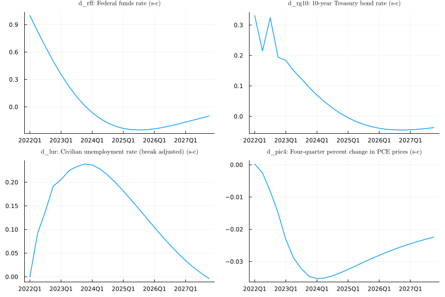
Simulate a shock
The last exercise is to simulate the impulse response to a unit shock in rffintay.
julia> m.rffintay"Value of eff. federal funds rate given by the inertial Taylor rule" rffintay
We start with the base case and add 1 to the rffintay_a shock at the first period of the simulation.
julia> p_1 = Plan(m, sim);julia> ed_1 = copy(sol_0);julia> ed_1.rffintay_a[first(sim)] += 1;julia> sol_1 = @time simulate(m, p_1, ed_1; verbose=true, tol=1e-9);[ Info: Simulating 2022Q1:2027Q4 [ Info: 1, || Fx || = 1.0, || Δx || = 5299.663208477447 [ Info: 2, || Fx || = 348.8940862391828, || Δx || = 337.83888249254574 [ Info: 3, || Fx || = 0.21547953275148757, || Δx || = 0.01265520208826992 [ Info: 4, || Fx || = 1.080850470458472e-5, || Δx || = 7.945683719180563e-7 [ Info: 5, || Fx || = 1.4551915228366852e-10 0.462913 seconds (1.21 M allocations: 167.899 MiB, 3.38% gc time)
Finally, we can plot the impulse response function to see what we've done.
julia> # compute the differences between the base case and the shocked simulation. dd = MVTSeries(p.range; d_rff=sol_1.rff - sol_0.rff, d_rg10=sol_1.rg10 - sol_0.rg10, d_lur=sol_1.lur - sol_0.lur, d_pic4=sol_1.pic4 - sol_0.pic4, );julia> # produce the plot plt = plot(dd, trange=sim, vars=(:d_rff, :d_rg10, :d_lur, :d_pic4), legend=false, size=(900, 600), linewidth=1.5, titlefontsize=8 );julia> plot!(plt[1,1], title="d_rff: $(m.rff.doc) (s-c)");julia> plot!(plt[1,2], title="d_rg10: $(m.rg10.doc) (s-c)");julia> plot!(plt[2,1], title="d_lur: $(m.lur.doc) (s-c)");julia> plot!(plt[2,2], title="d_pic4: $(m.pic4.doc) (s-c)");julia> pltPlot{Plots.GRBackend() n=4} Captured extra kwargs: Series{1}: trange: 2022Q1:2027Q4 vars: (:d_rff, :d_rg10, :d_lur, :d_pic4) Series{2}: trange: 2022Q1:2027Q4 vars: (:d_rff, :d_rg10, :d_lur, :d_pic4) Series{3}: trange: 2022Q1:2027Q4 vars: (:d_rff, :d_rg10, :d_lur, :d_pic4) Series{4}: trange: 2022Q1:2027Q4 vars: (:d_rff, :d_rg10, :d_lur, :d_pic4)