Time Series

In this tutorial we will see how to use the functionality provided in TimeSeriesEcon to manipulate time series data.

All code presented here is also available in main.jl.

Time Series

In this tutorial we need the following packages.

using TimeSeriesEcon
using Statistics
using Plots

Frequency and Time

In a time series the values are evenly spaced in time and each value is labelled with the moment in which it occurred. TimeSeriesEcon provides data types that represent these concepts.

The abstract type Frequency represents the idea of the frequency of a time series. All concrete frequencies are special cases. Currently we have four calendar frequencies, Yearly, HalfYearly, Quarterly, and Monthly, which are all defined by a number of periods per year. We have three calendar frequencies which depend on a particular calendar date: Weekly, BDaily and Daily. Finally We also have the frequency Unit, which is not based on the calendar and simply counts observations. Typically there's no need to work directly with these frequency types.

End-months and end-days

The frequencies Yearly, HalfYearly, and Quarterly have implicit default end months. These are 12, 6, and 3, respectively, corresponding to December, June and March. Uses of Yearly will in most cases implicitly use Yearly{12}. It is also possible to work with frequencies with different end months, for example, a fiscal year might end in March, in which case a Yearly{3} frequency would be used. These end months have implications for frequency conversions (not yet implemented), but can in most cases be ignored.

The Weekly frequency similarly has an implicit default end-day of Sunday. Thus uses of Weekly will in most cases implicitly use Weekly{7}.

Moments and Durations

In TimeSeriesEcon there are two data types to represent the notion of time. Data of type MIT are labels for particular moments in time, while the data type Duration represents the amount of time between two MITs. Both are generic types, in the sense that they are parametrized by a frequency. For example

julia> typeof(2000Q1)MIT{Quarterly{3}}
julia> typeof(2021M5 - 2020M3)Duration{Monthly}

Creating MIT instances

The most common types of MIT instances can be created using shorthands of numbers followed immediately by Y, H1, H2, Q1, Q2, Q3, or Q4. for example, the second half of 2022 would be 2022H2.

julia> 2022Q12022Q1
julia> 2022H12022H1
julia> 2020Q32020Q3
julia> 2020Y2020Y

For variant end-months, append these in square brackets:

julia> 2022Q1{2}2022Q1{2}
julia> 2022H1{5}2022H1{5}
julia> 2020Y{11}2020Y{11}

For the the higher frequencies, a Date object or string is required to create them:

julia> weekly("2022-01-03")2022-01-09
julia> bdaily("2022-01-03")2022-01-03
julia> daily("2022-01-03")2022-01-03

Creating a BDaily MIT from a date that lands on a weekend will throw an error, this can be overcome with passing the bias parameter. either :previous, :next, or :nearest.

julia> bdaily("2022-01-01", bias=:previous) # 2021-12-312021-12-31

Daily and bdaily frequencies can also be created using string macros:

julia> d"2022-01-03"2022-01-03
julia> bd"2022-01-03"2022-01-03
julia> bd"2022-01-01"p # 2021-12-312021-12-31
julia> bd"2022-01-01"n # 2022-01-032022-01-03

Arithmetic with Time

We can perform arithmetic operations with values of type MIT and Duration. We just saw that the difference of two MIT values is a Duration of the same frequency. Conversely, we can add an MIT and a Duration to get an MIT. We can add and subtract two Durations, but we're not allowed to add two MITs, only subtract them.

julia> a = 2001Q2 - 2000Q1  # the result is a Duration{Quarterly}5
julia> b = 2001Q2 + 2000Q1  # doesn't make sense!ERROR: ArgumentError: Illegal addition of two `MIT` values.

When we have an MIT plus or minus a plain Integer, the latter is automatically converted to a Duration of the appropriate frequency. This should make our code more readable.

julia> 2000Q1 + Duration{Quarterly}(6)  # this is clunky2001Q3
julia> 2000Q1 + 6 # same as above2001Q3

We're not allowed to mix frequencies.

julia> 2000Q1 + Duration{Monthly}(6)ERROR: ArgumentError: Mixing frequencies not allowed: Quarterly{3} and Monthly.

Other arithmetic operations involving MITs and Durations, either with each other or with Integers are not allowed.

julia> 2000Q1 * 5ERROR: ArgumentError: Invalid arithmetic operation with Int64 and MIT{Quarterly{3}}

Other Operations

The function frequencyof returns the frequency type of its argument.

julia> frequencyof(2000Y)Yearly{12}
julia> frequencyof(2020Q1 - 2019Q3)Quarterly{3}

There are a few operations which are valid only for calendar frequencies. The function ppy returns the number of periods, while TimeSeriesEcon.year and period return the year and the period number. The periods are numbered from 1 to ppy. If we need both, we can use mit2yp.

julia> t = 2020Q32020Q3
julia> ppy(t)4
julia> TimeSeriesEcon.year(t)2020
julia> period(t)3
julia> mit2yp(t)(2020, 3)

Note that ppy returns hardcoded numbers for weekly, daily, and bdaily frequencies, regardless of the actual year of the MIT passed. In addition, the TimeSeriesEcon.year, period, and mit2yp functions do not work for Weekly frequencies, due uncertainty surrounding weeks spanning the end of a year.

Ranges

We can create a range of MIT the same way we create ranges of integers. The standard Julia operations with ranges work on MIT ranges as well.

julia> rng = 2000M1:2001M92000M1:2001M9
julia> length(rng)21
julia> first(rng)2000M1
julia> last(rng)2001M9
julia> rng[3:5]   # subrange2000M3:2000M5
julia> rng .+ 6  # shift forward by 6 periods2000M7:2002M3

We can also create a range where the step is not 1 but some other integer. Technically the step should be a Duration, but once again we can use an Integer for convenience.

julia> rng2 = 2000M1:2:2000M82000M1:2:2000M7
julia> collect(rng2)4-element Vector{MIT{Monthly}}:
 2000M1
 2000M3
 2000M5
 2000M7

We can create a range that runs backwards by swapping the endpoints and making the step -1. But it is easier to call the standard Julia function reverse. This can be helpful when using @rec as shown below.

julia> rng2000M1:2001M9
julia> reverse(rng)2001M9:-1:2000M1

We can also use the string macros to create ranges of Daily and BDaily frequencies. When creating a BDaily range in this way, the first date will be rounded up and the last date rounded down whenever these fall on a weekend.

julia> d"2022-01-01:2022-01-31"Daily 2022-01-01:2022-01-31
julia> bd"2022-01-01:2022-01-31"BDaily 2022-01-03:2022-01-31

Time Series

TimeSeriesEcon provides the data type TSeries to represent a macro-economic time series. It is similar to a Vector, but with added functionality for time series.

The TSeries type inherits from the built-in AbstractArray and supports all the basic operations of 1-dimensional arrays in Julia. Refer to the article on Multi-dimensional Arrays in the Julia manual for details.

Type TSeries is also a generic data type. It depends on two type-parameters: its frequency and the data type of its elements.

Creation of `TSeries`

Constructors

The basic constructor of a TSeries requires an MIT (to label the first observation) and a vector of data.

julia> vals = rand(5)5-element Vector{Float64}:
 0.2432776234150773
 0.05880174455980336
 0.12803258393507333
 0.8198455071246772
 0.2616461870532787
julia> ts = TSeries(2020Q1, vals)5-element TSeries{Quarterly} with range 2020Q1:2021Q1:
  2020Q1 : 0.2432776234150773
  2020Q2 : 0.05880174455980336
  2020Q3 : 0.12803258393507333
  2020Q4 : 0.8198455071246772
  2021Q1 : 0.2616461870532787

The frequency of the given MIT determines the frequency of the TSeries. Similarly, the type of the elements of the vals array determines the element type of the TSeries.

Important Caveat

Be mindful of the fact that the TSeries does not copy the original data container. Rather, the ts constructed above is just a wrapper and uses vals for its storage. Specifically, every modification to one of them is immediately reflected in the other. To break the connection use copy.

ts = TSeries(2020Q1, copy(vals))

We can construct a TSeries with its own storage from just an MIT range. This would construct a TSeries whose storage is un-initialized (it would contain some arbitrary numbers). We can initialize the storage by providing a constant or a function, such as zeros, ones, rand.

julia> rng = 2020Q1:2021Q42020Q1:2021Q4
julia> TSeries(rng)  # uninitialized (arbitrary numbers that happen to be in memory)8-element TSeries{Quarterly} with range 2020Q1:2021Q4:
  2020Q1 : 0.0
  2020Q2 : 0.0
  2020Q3 : 0.0
  2020Q4 : 0.0
  2021Q1 : 0.0
  2021Q2 : 0.0
  2021Q3 : 0.0
  2021Q4 : 0.0
julia> TSeries(rng, pi)    # constant8-element TSeries{Quarterly,Irrational{:π}} with range 2020Q1:2021Q4:
  2020Q1 : π
  2020Q2 : π
  2020Q3 : π
  2020Q4 : π
  2021Q1 : π
  2021Q2 : π
  2021Q3 : π
  2021Q4 : π
julia> TSeries(rng, rand)  # random numbers8-element TSeries{Quarterly} with range 2020Q1:2021Q4:
  2020Q1 : 0.9756910609790161
  2020Q2 : 0.8887513238044153
  2020Q3 : 0.440092854420851
  2020Q4 : 0.530739351242023
  2021Q1 : 0.8980822001220053
  2021Q2 : 0.6608538795937574
  2021Q3 : 0.6995576397827303
  2021Q4 : 0.6472088561522328

Important

Be mindful of the type of the constant you provide as initializer. Specifically, in Julia 0 is of type Int while 0.0 is of type Float64. If you're never going to work with TSeries that store integers (most people), then we recommend you get used to the idiom TSeries(rng, zeros), which does what you expect.

TSeries(rng,0)   # element type is Int
TSeries(rng, zeros) # element type is FLoat64

Other ways to construct `TSeries`

We can also construct new TSeries from existing TSeries. The function similar(::TSeries) creates an uninitialized copy, meaning that the copy has the same frequency and element type, but the storage contains arbitrary values. This is useful if we just want a TSeries that we will fill in later. The other useful function is copy, which makes an exact copy. In both cases the new and the old TSeries have separate storage.

julia> t = TSeries(rng, 2.7)8-element TSeries{Quarterly} with range 2020Q1:2021Q4:
  2020Q1 : 2.7
  2020Q2 : 2.7
  2020Q3 : 2.7
  2020Q4 : 2.7
  2021Q1 : 2.7
  2021Q2 : 2.7
  2021Q3 : 2.7
  2021Q4 : 2.7
julia> s = similar(t)8-element TSeries{Quarterly} with range 2020Q1:2021Q4:
  2020Q1 : 6.93450407376164e-310
  2020Q2 : 6.93450365252996e-310
  2020Q3 : 6.9345421126421e-310
  2020Q4 : 6.9345311885807e-310
  2021Q1 : 6.9345421126421e-310
  2021Q2 : 6.9345421126421e-310
  2021Q3 : 5.0e-324
  2021Q4 : NaN
julia> c = copy(t)8-element TSeries{Quarterly} with range 2020Q1:2021Q4:
  2020Q1 : 2.7
  2020Q2 : 2.7
  2020Q3 : 2.7
  2020Q4 : 2.7
  2021Q1 : 2.7
  2021Q2 : 2.7
  2021Q3 : 2.7
  2021Q4 : 2.7

New TSeries are also the results of arithmetic and other operation, which we discuss later in this tutorial.

Access to Elements of `TSeries`

Reading (Indexing)

We can access the value for a specific MIT using the standard indexing notation in Julia.

julia> rng = 2000Q1:2001Q1;
julia> t = TSeries(rng, rand)5-element TSeries{Quarterly} with range 2000Q1:2001Q1:
  2000Q1 : 0.5216738029820028
  2000Q2 : 0.26890562996573697
  2000Q3 : 0.17063052088218034
  2000Q4 : 0.45874147265491416
  2001Q1 : 0.3044727318627928
julia> t[2000Q1]0.5216738029820028

If we ask for a range of MIT, the result is a new TSeries.

julia> t[2000Q2:2000Q4]3-element TSeries{Quarterly} with range 2000Q2:2000Q4:
  2000Q2 : 0.26890562996573697
  2000Q3 : 0.17063052088218034
  2000Q4 : 0.45874147265491416

We can also use integers. In this case the TSeries behaves like a Vector. The valid integer bounds are 1:length(ts). Note that if we use an integer range, the result is a Vector, not a TSeries.

julia> t[1]0.5216738029820028
julia> t[2:4]3-element Vector{Float64}:
 0.26890562996573697
 0.17063052088218034
 0.45874147265491416

If we attempt to read outside the stored range, we would get a BoundsError, which is the same for Vectors.

julia> t[1999Q1]ERROR: BoundsError: attempt to access 5-element TSeries{Quarterly} with range 2000Q1:2001Q1 at index [1999Q1]
julia> t[2001Q1:2001Q3]ERROR: BoundsError: attempt to access 5-element TSeries{Quarterly} with range 2000Q1:2001Q1 at index [2001Q1:2001Q3]

When specifying a range, we can use begin and end inside the []. This works exactly the same way for TSeries as it does for the built-in Vector.

julia> t[end-2:end]   # last 33-element TSeries{Quarterly} with range 2000Q3:2001Q1:
  2000Q3 : 0.17063052088218034
  2000Q4 : 0.45874147265491416
  2001Q1 : 0.3044727318627928
julia> t[begin+1:end-1]  # drop first and last3-element TSeries{Quarterly} with range 2000Q2:2000Q4:
  2000Q2 : 0.26890562996573697
  2000Q3 : 0.17063052088218034
  2000Q4 : 0.45874147265491416

Important

Keep in mind that begin and end for TSeries are of type MIT. Specifically, when using them we must make sure that both limits of the range evaluate to MIT and not integer. For example, julia ts[1:end-1] # error will result in an error because the first limit is 1, an Int, while the last limit is lastdate(ts)-1, an MIT). To make this work we need this. julia ts[begin:end-1] # correct

Writing (Indexed Assignment)

When indexing is used on the left side of an assignment, we're updating the specified element(s) of the TSeries. Again, this works the same as with Vectors.

julia> t[2000Q2] = 55
julia> t5-element TSeries{Quarterly} with range 2000Q1:2001Q1:
  2000Q1 : 0.5216738029820028
  2000Q2 : 5.0
  2000Q3 : 0.17063052088218034
  2000Q4 : 0.45874147265491416
  2001Q1 : 0.3044727318627928

When assigning to multiple locations (e.g., over a range), we must ensure that the number of values provided on the right-hand side is correct. Otherwise we would get an error.

julia> t[begin:begin + 2] = [1, 2, 3]3-element Vector{Int64}:
 1
 2
 3
julia> t5-element TSeries{Quarterly} with range 2000Q1:2001Q1:
  2000Q1 : 1.0
  2000Q2 : 2.0
  2000Q3 : 3.0
  2000Q4 : 0.45874147265491416
  2001Q1 : 0.3044727318627928

If we want to assign a single value to multiple locations we have to make the assignment a vectorized "dot" operation. For this we use .= instead of =.

julia> t[end-2:end] .= 423-element TSeries{Quarterly} with range 2000Q3:2001Q1:
  2000Q3 : 42.0
  2000Q4 : 42.0
  2001Q1 : 42.0
julia> t5-element TSeries{Quarterly} with range 2000Q1:2001Q1:
  2000Q1 : 1.0
  2000Q2 : 2.0
  2000Q3 : 42.0
  2000Q4 : 42.0
  2001Q1 : 42.0

The same way we can reset the entire TSeries to a constant using .= without specifying the range. This would update the existing TSeries in place.

julia> t .= pi5-element TSeries{Quarterly} with range 2000Q1:2001Q1:
  2000Q1 : 3.141592653589793
  2000Q2 : 3.141592653589793
  2000Q3 : 3.141592653589793
  2000Q4 : 3.141592653589793
  2001Q1 : 3.141592653589793

Without the dot, i.e., t = pi, t would become a completely different variable with value pi.

Unlike Vectors, with TSeries we are allowed to assign outside the stored range. Doing this resizes the TSeries as necessary. If there is a gap, that is a part of the new range which is neither in the old range nor in the assignment range, it is filled with NaN.

julia> t[1999Q1:1999Q2] .= -3.72-element TSeries{Quarterly} with range 1999Q1:1999Q2:
  1999Q1 : -3.7
  1999Q2 : -3.7
julia> t9-element TSeries{Quarterly} with range 1999Q1:2001Q1:
  1999Q1 : -3.7
  1999Q2 : -3.7
  1999Q3 : NaN
  1999Q4 : NaN
  2000Q1 : 3.141592653589793
  2000Q2 : 3.141592653589793
  2000Q3 : 3.141592653589793
  2000Q4 : 3.141592653589793
  2001Q1 : 3.141592653589793

This only works with MIT indexing. If an integer index is out of bounds, the attempted assignment will result in the usual BoundsError, which is what we would get with a Vector.

julia> t[15] = 3.5   # results in an errorERROR: BoundsError: attempt to access 9-element Vector{Float64} at index [15]

The vectorized "dot" assignment allows us to copy values from another TSeries. In this case, the specified range on the left of .= applies to the right side too. In other words, the values from the right hand side will be taken from the range of the assignment.

julia> q = TSeries(rangeof(t), 100)9-element TSeries{Quarterly,Int64} with range 1999Q1:2001Q1:
  1999Q1 : 100
  1999Q2 : 100
  1999Q3 : 100
  1999Q4 : 100
  2000Q1 : 100
  2000Q2 : 100
  2000Q3 : 100
  2000Q4 : 100
  2001Q1 : 100
julia> t[1999Q3:2000Q2] .= q4-element TSeries{Quarterly} with range 1999Q3:2000Q2:
  1999Q3 : 100.0
  1999Q4 : 100.0
  2000Q1 : 100.0
  2000Q2 : 100.0
julia> t9-element TSeries{Quarterly} with range 1999Q1:2001Q1:
  1999Q1 : -3.7
  1999Q2 : -3.7
  1999Q3 : 100.0
  1999Q4 : 100.0
  2000Q1 : 100.0
  2000Q2 : 100.0
  2000Q3 : 3.141592653589793
  2000Q4 : 3.141592653589793
  2001Q1 : 3.141592653589793

Arithmetic with `TSeries`

There are two kinds of arithmetic operations with TSeries. One kind is where we treat the time series as a single object. Similarly to vectors, we have addition of time series and multiplication of a time series by a scalar number. The other kind of arithmetic is where we treat the time series as a collection of numbers and do the operations element-wise.

In both cases, if there are multiple time series involved in an expression they must all be of the same frequency, otherwise the operation is generally not well defined.

When we add (or subtract) two or more TSeries their ranges are not required to be identical. The resulting TSeries has a range containing the common part of all ranges. This is in spirit with the idea that we treat values of a time series outside of its range as unknown or missing, so the result of arithmetic with unknown values remains unknown.

julia> x = TSeries(20Q1:20Q4, rand)4-element TSeries{Quarterly} with range 20Q1:20Q4:
  20Q1 : 0.2703093357786882
  20Q2 : 0.6960854934014918
  20Q3 : 0.8948884857965246
  20Q4 : 0.6191898125656232
julia> y = TSeries(20Q3:21Q2, rand)4-element TSeries{Quarterly} with range 20Q3:21Q2:
  20Q3 : 0.1810140910642123
  20Q4 : 0.30941879513917325
  21Q1 : 0.4428612328751693
  21Q2 : 0.4627658914910493
julia> x + y2-element TSeries{Quarterly} with range 20Q3:20Q4:
  20Q3 : 1.0759025768607369
  20Q4 : 0.9286086077047965
julia> x - y2-element TSeries{Quarterly} with range 20Q3:20Q4:
  20Q3 : 0.7138743947323123
  20Q4 : 0.30977101742644997

When we multiply (or divide) a TSeries by a scalar the resulting TSeries has the same range as the original.

julia> 2y4-element TSeries{Quarterly} with range 20Q3:21Q2:
  20Q3 : 0.3620281821284246
  20Q4 : 0.6188375902783465
  21Q1 : 0.8857224657503386
  21Q2 : 0.9255317829820986
julia> y/24-element TSeries{Quarterly} with range 20Q3:21Q2:
  20Q3 : 0.09050704553210615
  20Q4 : 0.15470939756958663
  21Q1 : 0.22143061643758466
  21Q2 : 0.23138294574552465

For element-wise operations we use Julia's "dot" notation. This notation is used for vectorized and broadcasting operations. The time series are aligned so that element-wise operations are performed on matching MIT across all TSeries in the expression. For this reason, once again, they all must have the same frequency and the range of the result is the intersection of all ranges.

julia> log.(x)   # use dot for vectorized function call4-element TSeries{Quarterly} with range 20Q1:20Q4:
  20Q1 : -1.3081882877142759
  20Q2 : -0.36228279084438986
  20Q3 : -0.11105616534550872
  20Q4 : -0.4793434094168627
julia> 1 .+ x    # broadcasting addition of scalar 1 to time series x4-element TSeries{Quarterly} with range 20Q1:20Q4:
  20Q1 : 1.270309335778688
  20Q2 : 1.6960854934014917
  20Q3 : 1.8948884857965247
  20Q4 : 1.6191898125656232
julia> x .+ y    # vectorized addition (same as regular addition of TSeries)2-element TSeries{Quarterly} with range 20Q3:20Q4:
  20Q3 : 1.0759025768607369
  20Q4 : 0.9286086077047965
julia> 2 ./ y    # broadcasting division division4-element TSeries{Quarterly} with range 20Q3:21Q2:
  20Q3 : 11.048863589799355
  20Q4 : 6.463731458525076
  21Q1 : 4.516087323822599
  21Q2 : 4.321839696430357
julia> y .^ 3    # broadcasting y-cubed4-element TSeries{Quarterly} with range 20Q3:21Q2:
  20Q3 : 0.005931126019883818
  20Q4 : 0.029623752595447105
  21Q1 : 0.08685663386052772
  21Q2 : 0.09910236629294032

When assigning the result of a broadcasting operation within an existing TSeries we have to use .= and may optionally specify a range on the left-hand side. When we specify a range on the left-hand side the TSeries on the left is resized, if necessary, to include the given range.

julia> z = copy(x)4-element TSeries{Quarterly} with range 20Q1:20Q4:
  20Q1 : 0.2703093357786882
  20Q2 : 0.6960854934014918
  20Q3 : 0.8948884857965246
  20Q4 : 0.6191898125656232
julia> z .=  1 .+ y  # assign only within the common range of x and y4-element TSeries{Quarterly} with range 20Q1:20Q4:
  20Q1 : 0.2703093357786882
  20Q2 : 0.6960854934014918
  20Q3 : 1.1810140910642124
  20Q4 : 1.3094187951391731
julia> z4-element TSeries{Quarterly} with range 20Q1:20Q4:
  20Q1 : 0.2703093357786882
  20Q2 : 0.6960854934014918
  20Q3 : 1.1810140910642124
  20Q4 : 1.3094187951391731
julia> z[rangeof(y)] .= 3 .+ y  # resize x and assign within the full range of y4-element TSeries{Quarterly} with range 20Q3:21Q2:
  20Q3 : 3.1810140910642124
  20Q4 : 3.309418795139173
  21Q1 : 3.4428612328751695
  21Q2 : 3.462765891491049
julia> z6-element TSeries{Quarterly} with range 20Q1:21Q2:
  20Q1 : 0.2703093357786882
  20Q2 : 0.6960854934014918
  20Q3 : 3.1810140910642124
  20Q4 : 3.309418795139173
  21Q1 : 3.4428612328751695
  21Q2 : 3.462765891491049

Broadcasting operations also can be done with mixing TSeries and Vectors in the same expression. In this case, the Vector must be of the same length as the TSeries and the result is a TSeries.

julia> v = 3ones(size(x))4-element Vector{Float64}:
 3.0
 3.0
 3.0
 3.0
julia> x .+ v4-element TSeries{Quarterly} with range 20Q1:20Q4:
  20Q1 : 3.270309335778688
  20Q2 : 3.6960854934014917
  20Q3 : 3.8948884857965247
  20Q4 : 3.619189812565623

Time Series Operations

Shifts

The lag or lead of a TSeries is an operation where the data remains the same but the MIT labels are shifted accordingly. Functions lag and lead produce a new TSeries, while lag! and lead! modify the given TSeries in place. A second integer argument n can be provided to indicate which lag or lead is desired, if something other than 1.

julia> lag(x)4-element TSeries{Quarterly} with range 20Q2:21Q1:
  20Q2 : 0.2703093357786882
  20Q3 : 0.6960854934014918
  20Q4 : 0.8948884857965246
  21Q1 : 0.6191898125656232
julia> lead(x)4-element TSeries{Quarterly} with range 19Q4:20Q3:
  19Q4 : 0.2703093357786882
  20Q1 : 0.6960854934014918
  20Q2 : 0.8948884857965246
  20Q3 : 0.6191898125656232

Diff and Undiff

The first difference of a TSeries can be computed with the built-in function diff. The built-in version works for any Vector, including TSeries. In addition, for time series version of diff allows a second integer argument k to indicate which lag or lead to subtract. The default is k=-1, where a negative value of k indicates a lag and a positive value indicates a lead.

julia> dx = diff(x)3-element TSeries{Quarterly} with range 20Q2:20Q4:
  20Q2 : 0.42577615762280363
  20Q3 : 0.19880299239503274
  20Q4 : -0.27569867323090136

The inverse operation can be done with the function undiff. In its basic form it is the same as the built-in function cumsum.

julia> undiff(dx)4-element TSeries{Quarterly} with range 20Q1:20Q4:
  20Q1 : 0.0
  20Q2 : 0.42577615762280363
  20Q3 : 0.6245791500178364
  20Q4 : 0.348880476786935

We can see that the answer above does not equal x. This is because the first value of x was lost. undiff allows us to specify an "anchor" in the form of date => value. In this case the resulting TSeries will have the given value at the given date.

julia> x2 = undiff(dx, firstdate(x) => first(x))4-element TSeries{Quarterly} with range 20Q1:20Q4:
  20Q1 : 0.2703093357786882
  20Q2 : 0.6960854934014918
  20Q3 : 0.8948884857965246
  20Q4 : 0.6191898125656232
julia> x ≈ x2true

Good to know

In the call to undiff above we used first, which is a built-in Julia function that returns the first value of a collection. We also used firstdate, which works for TSeries and returns the first date in the stored range of its argument.

Moving Average

Moving average can be computed with a call to the function moving. It takes a second integer argument n which indicates the length of the window over which the moving average will be computed. If n is positive, the window is backwards-looking (includes lags), while negative n uses a forward-looking window (includes leads). The window always includes the current value (lag 0).

julia> tt = TSeries(2020Q1, collect(Float64, 1:10))10-element TSeries{Quarterly} with range 2020Q1:2022Q2:
  2020Q1 : 1.0
  2020Q2 : 2.0
  2020Q3 : 3.0
  2020Q4 : 4.0
  2021Q1 : 5.0
  2021Q2 : 6.0
  2021Q3 : 7.0
  2021Q4 : 8.0
  2022Q1 : 9.0
  2022Q2 : 10.0
julia> moving(tt, -4)7-element TSeries{Quarterly} with range 2020Q1:2021Q3:
  2020Q1 : 2.5
  2020Q2 : 3.5
  2020Q3 : 4.5
  2020Q4 : 5.5
  2021Q1 : 6.5
  2021Q2 : 7.5
  2021Q3 : 8.5
julia> moving(tt, 6)5-element TSeries{Quarterly} with range 2021Q2:2022Q2:
  2021Q2 : 3.5
  2021Q3 : 4.5
  2021Q4 : 5.5
  2022Q1 : 6.5
  2022Q2 : 7.5

Recursive assignments

Sometimes we need to construct a time series by recursive assignments. We can do this on one line with the macro @rec. For example, we can simulate the impulse response of a simple AR(1) model. Say math a_t = (1-\rho) a_{ss} + \rho a_{t-1} + \varepsilon_t. Then we can compute the impulse response with the following snippet of code.

julia> a_ss = 1.01.0
julia> ρ = 0.60.6
julia> a = fill(a_ss, 2020Q1:2022Q1)9-element TSeries{Quarterly} with range 2020Q1:2022Q1:
  2020Q1 : 1.0
  2020Q2 : 1.0
  2020Q3 : 1.0
  2020Q4 : 1.0
  2021Q1 : 1.0
  2021Q2 : 1.0
  2021Q3 : 1.0
  2021Q4 : 1.0
  2022Q1 : 1.0
julia> a[begin] += 0.11.1
julia> for t = firstdate(a)+1:lastdate(a)
           a[t] = (1-ρ)*a_ss + ρ*a[t-1]
       end
julia> a9-element TSeries{Quarterly} with range 2020Q1:2022Q1:
  2020Q1 : 1.1
  2020Q2 : 1.06
  2020Q3 : 1.036
  2020Q4 : 1.0216
  2021Q1 : 1.01296
  2021Q2 : 1.007776
  2021Q3 : 1.0046656
  2021Q4 : 1.00279936
  2022Q1 : 1.001679616

We can rewrite the last loop more succinctly like this:

julia> @rec rangeof(a, drop=1) a[t] = (1-ρ)*a_ss + ρ*a[t-1]
julia> a9-element TSeries{Quarterly} with range 2020Q1:2022Q1:
  2020Q1 : 1.1
  2020Q2 : 1.06
  2020Q3 : 1.036
  2020Q4 : 1.0216
  2021Q1 : 1.01296
  2021Q2 : 1.007776
  2021Q3 : 1.0046656
  2021Q4 : 1.00279936
  2022Q1 : 1.001679616

The first argument of @rec is the range over which the loop will run. In this case we're using rangeof(a, drop=1). Function rangeof normally returns the stored range of a TSeries. With the optional parameter drop=n we request that the first n periods be skipped. If n is negative, then the periods will be skipped at the end.

julia> (rangeof(a), rangeof(a, drop=1), rangeof(a, drop=-1))(2020Q1:2022Q1, 2020Q2:2022Q1, 2020Q1:2021Q4)

Note also that whether using @rec or spelling out the for-loop explicitly, the TSeries will be resized if necessary. However, it is more efficient to preallocate the entire range by calling resize! first.

julia> resize!(a, 2020Q1:2023Q1)13-element TSeries{Quarterly} with range 2020Q1:2023Q1:
  2020Q1 : 1.1
  2020Q2 : 1.06
  2020Q3 : 1.036
  2020Q4 : 1.0216
  2021Q1 : 1.01296
  2021Q2 : 1.007776
  2021Q3 : 1.0046656
  2021Q4 : 1.00279936
  2022Q1 : 1.001679616
  2022Q2 : NaN
  2022Q3 : NaN
  2022Q4 : NaN
  2023Q1 : NaN
julia> @rec rangeof(a, drop=1) a[t] = (1-ρ)*a_ss + ρ*a[t-1]
julia> a13-element TSeries{Quarterly} with range 2020Q1:2023Q1:
  2020Q1 : 1.1
  2020Q2 : 1.06
  2020Q3 : 1.036
  2020Q4 : 1.0216
  2021Q1 : 1.01296
  2021Q2 : 1.007776
  2021Q3 : 1.0046656
  2021Q4 : 1.00279936
  2022Q1 : 1.001679616
  2022Q2 : 1.0010077696000002
  2022Q3 : 1.0006046617600002
  2022Q4 : 1.000362797056
  2023Q1 : 1.0002176782336

Multi-variate Time Series

We can store multiple time series in a variable of type MVTSeries. This is a collection of TSeries with the same frequency, the same range, and the same element type. It is like a table, where each row corresponds to an MIT and each column to a time series variable.

Creation of `MVTSeries`

The basic constructor of MVTSeries takes an MIT, which indicates the label of the first row, a list of names for the columns, and a matrix of values. The number of columns in the given matrix must match the number of column names. The range of the resulting MVTSeries is determined from the first date and the number of rows.

julia> x = MVTSeries(2020Q1, (:a, :b), rand(6, 2))6×2 MVTSeries{Quarterly} with range 2020Q1:2021Q2 and variables (a,b):
           a         b
  2020Q1 : 0.413248  0.288845
  2020Q2 : 0.753866  0.379668
  2020Q3 : 0.837555  0.29682
  2020Q4 : 0.465706  0.935465
  2021Q1 : 0.885335  0.484721
  2021Q2 : 0.461721  0.67609

Similarly to TSeries, if we specify a range (rather than a single MIT), the MVTSeries will be able to allocate its own storage. In this case, we can optionally provide an initializer in the form of a constant value or a function.

julia> MVTSeries(2020Q1:2021Q3, (:one, :too, :tree), zeros)7×3 MVTSeries{Quarterly} with range 2020Q1:2021Q3 and variables (one,too,…):
           one     too     tree
  2020Q1 : 0.0     0.0     0.0
  2020Q2 : 0.0     0.0     0.0
  2020Q3 : 0.0     0.0     0.0
  2020Q4 : 0.0     0.0     0.0
  2021Q1 : 0.0     0.0     0.0
  2021Q2 : 0.0     0.0     0.0
  2021Q3 : 0.0     0.0     0.0

We can also build an MVTSeries from a range and a list of name-value pairs. The values can be TSeries, vectors, or constants. In the case of a TSeries, the constructor will use the necessary range, while in the case of a vector must have the correct length. This form of the MVTSeries constructor allocates its own storage space, so the data are always copied.

julia> data = MVTSeries(2020Q1:2021Q1;
                   hex = TSeries(2019Q1, collect(Float64, 1:20)),
                   why = zeros(5),
                   zed = 3, )5×3 MVTSeries{Quarterly} with range 2020Q1:2021Q1 and variables (hex,why,…):
           hex     why     zed
  2020Q1 : 5.0     0.0     3.0
  2020Q2 : 6.0     0.0     3.0
  2020Q3 : 7.0     0.0     3.0
  2020Q4 : 8.0     0.0     3.0
  2021Q1 : 9.0     0.0     3.0

New MVTSeries variables can also be created with similar(::MVTSeries) and copy. They are also the result of arithmetic operations. This is the same as with TSeries, so we won't spend time repeating it.

Access

MVTSeries behaves like a 2-dimensional matrix when indexing is done with integers. Otherwise, we can also index using MITs (or MIT ranges) for the row-indexes and Symbols (or tuples of Symbols) for the column-indexes.

julia> data[2020Q2, :hex]6.0

An entire row can be accessed with a single MIT index. The result of such indexing is a regular Vector. In order to extract an MVTSeries the index must be a unit range of MIT.

julia> data[2020Q2]3-element Vector{Float64}:
 6.0
 0.0
 3.0
julia> data[2020Q2:2020Q2]  # index with range1×3 MVTSeries{Quarterly} with range 2020Q2:2020Q2 and variables (hex,why,…):
           hex     why     zed
  2020Q2 : 6.0     0.0     3.0

Similarly, we can extract an entire column by its name. The result is a TSeries. If the index is a tuple of names, then the result is another MVTSeries containing only the selected columns.

julia> data[:zed]5-element TSeries{Quarterly} with range 2020Q1:2021Q1:
  2020Q1 : 3.0
  2020Q2 : 3.0
  2020Q3 : 3.0
  2020Q4 : 3.0
  2021Q1 : 3.0
julia> data[(:zed,)] # index with tuple5×1 MVTSeries{Quarterly} with range 2020Q1:2021Q1 and variables (zed):
           zed
  2020Q1 : 3.0
  2020Q2 : 3.0
  2020Q3 : 3.0
  2020Q4 : 3.0
  2021Q1 : 3.0

For convenience we can also access the columns by name using the traditional data.zed notation.

data.zed

It is sometimes necessary to iterate over the columns of an MVTSeries. This can be done easily with the function columns. The following snippet of code shows an idiom for such iteration.

julia> using Statistics
julia> for (name, value) in columns(data)
           println("Average of `", name, "` is ", mean(value), ".")
       endAverage of `hex` is 7.0.
Average of `why` is 0.0.
Average of `zed` is 3.0.

Note

Note that columns is specific to MVTSeries. The built-in function pairs does the same for a general collection of name-value pairs. It also works for MVTSeries.

Plotting

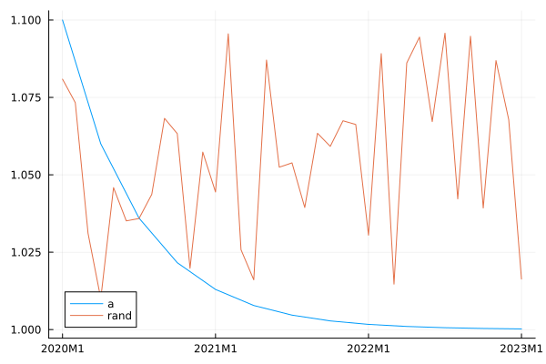
Visualizing a TSeries is straight-forward.

julia> plot(a, 1 .+ 0.1*TSeries(2020M1:2023M1, rand), label=["a" "rand"]);

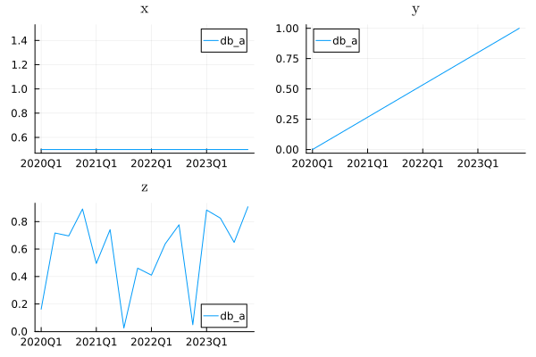
Similarly, we can plot all time series in an MVTSeries just as easily. Each variable will appear in its own set of axes.

julia> db_a = MVTSeries(2020Q1:2023Q4,
           x = 0.5,
           y = 0:1/15:1,
           z = rand(16),
       )16×3 MVTSeries{Quarterly} with range 2020Q1:2023Q4 and variables (x,y,z):
           x     y          z
  2020Q1 : 0.5   0.0        0.162018
  2020Q2 : 0.5   0.0666667  0.716907
  2020Q3 : 0.5   0.133333   0.695714
  2020Q4 : 0.5   0.2        0.891802
  2021Q1 : 0.5   0.266667   0.494901
  2021Q2 : 0.5   0.333333   0.741697
  2021Q3 : 0.5   0.4        0.0247565
  2021Q4 : 0.5   0.466667   0.460842
  2022Q1 : 0.5   0.533333   0.409918
  2022Q2 : 0.5   0.6        0.638017
  2022Q3 : 0.5   0.666667   0.776631
  2022Q4 : 0.5   0.733333   0.0487003
  2023Q1 : 0.5   0.8        0.884293
  2023Q2 : 0.5   0.866667   0.825299
  2023Q3 : 0.5   0.933333   0.648705
  2023Q4 : 0.5   1.0        0.907848
julia> plot(db_a, label=["db_a"]);

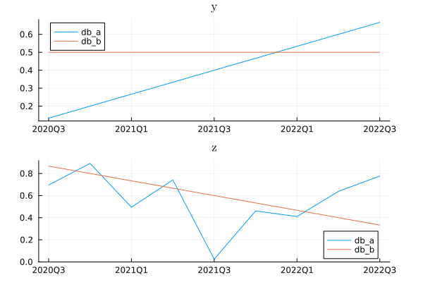
We cal also plot several MVTSeries at the same time.

julia> db_b = MVTSeries(2020Q1:2023Q4,
           y = 0.5,
           z = 1:-1/15:0,
           w = rand(16),
       )16×3 MVTSeries{Quarterly} with range 2020Q1:2023Q4 and variables (y,z,w):
           y     z          w
  2020Q1 : 0.5   1.0        0.34848
  2020Q2 : 0.5   0.933333   0.451829
  2020Q3 : 0.5   0.866667   0.10748
  2020Q4 : 0.5   0.8        0.787117
  2021Q1 : 0.5   0.733333   0.24017
  2021Q2 : 0.5   0.666667   0.235446
  2021Q3 : 0.5   0.6        0.373138
  2021Q4 : 0.5   0.533333   0.729125
  2022Q1 : 0.5   0.466667   0.314388
  2022Q2 : 0.5   0.4        0.137058
  2022Q3 : 0.5   0.333333   0.0606878
  2022Q4 : 0.5   0.266667   0.303859
  2023Q1 : 0.5   0.2        0.477063
  2023Q2 : 0.5   0.133333   0.495122
  2023Q3 : 0.5   0.0666667  0.771898
  2023Q4 : 0.5   0.0        0.103599
julia> plot(db_a, db_b, label=["db_a" "db_b"]);

We see that all variables are plotted as long as they appear in at least one of the given MVTSeries. The plot can become very busy very quickly. There is also a limit of 10 variables (which will result in a 5$\times$2 grid). We can select which variables to plot with the option vars=. We can also restrict the range of the plot with trange=. Any other plot attributes work as usual.

julia> plot(db_a, db_b,
           label = ["db_a" "db_b"],
           vars = [:y, :z],
           trange = 2020Q3:2022Q3,
           layout = (2,1),
       );

Good to Know

The trange= argument works only when all time series in the plot have the same frequency. When plotting time series with different frequencies, you can use xlim=. You can use MIT in the limits specified by xlim

they are converted to floating point numbers automatically. For example float(2020Q1) == 2020.0, float(2020Q2) = 2020.25, etc. An important difference to keep in mind is that trange= requires a unit range, e.g., trange=2020Q3:2022Q3, while xlim= requires a tuple, e.g., xlim=(2020Q3,2022Q3).

`Workspace`s

When working with models, in addition to time series data, we encounter a lot of other types of data. For example, parameter and steady state values, simulation ranges and dates, etc. The data type Workspace is a container that can store all kinds of data. Most operations for dictionaries work also for Workspaces.

We can create an empty Workspace and fill it with data. We can create "variables" in the workspace directly by assignment.

julia> w = Workspace()Empty Workspace
julia> w.rng = 2020Q1:2021Q42020Q1:2021Q4
julia> w.start = first(w.rng)2020Q1
julia> w.a = TSeries(w.rng)8-element TSeries{Quarterly} with range 2020Q1:2021Q4:
  2020Q1 : 3.0e-323
  2020Q2 : 3.5e-323
  2020Q3 : 4.0e-323
  2020Q4 : 4.4e-323
  2021Q1 : 4.4e-323
  2021Q2 : 5.4e-323
  2021Q3 : 5.4e-323
  2021Q4 : 3.5e-323
julia> w.a .= a8-element TSeries{Quarterly} with range 2020Q1:2021Q4:
  2020Q1 : 1.1
  2020Q2 : 1.06
  2020Q3 : 1.036
  2020Q4 : 1.0216
  2021Q1 : 1.01296
  2021Q2 : 1.007776
  2021Q3 : 1.0046656
  2021Q4 : 1.00279936
julia> wWorkspace with 3 variables
    rng ⇒ 2020Q1:2021Q4
  start ⇒ 2020Q1
      a ⇒ 8-element TSeries{Quarterly} with range 2020Q1:2021Q4

We can remove data from the workspace using the built-in function delete!.

julia> delete!(w, :start)Workspace with 2 variables
  rng ⇒ 2020Q1:2021Q4
    a ⇒ 8-element TSeries{Quarterly} with range 2020Q1:2021Q4

We can also give the constructor of Workspace a list of names and values like this:

julia> Workspace(rng = 2020Q1:2021Q4, alpha = 0.1, v = TSeries(2020Q1, rand(6)))Workspace with 3 variables
    rng ⇒ 2020Q1:2021Q4
  alpha ⇒ 0.1
      v ⇒ 6-element TSeries{Quarterly} with range 2020Q1:2021Q2

Equivalently, we can provide the whole list of name-value pairs as a single argument:

julia> datalist = [:rng => 2020Q1:2021Q4, :alpha => 0.1, :v => TSeries(2020Q1, rand(6))]3-element Vector{Pair{Symbol, Any}}:
   :rng => 2020Q1:2021Q4
 :alpha => 0.1
     :v => 6-element TSeries{Quarterly} with range 2020Q1:2021Q2:
  2020Q1 : 0.7940369211069682
  2020Q2 : 0.43061110867154906
  2020Q3 : 0.4446931668009563
  2020Q4 : 0.9592912754445723
  2021Q1 : 0.8759902224967694
  2021Q2 : 0.7863296147386446
julia> Workspace(datalist)Workspace with 3 variables
    rng ⇒ 2020Q1:2021Q4
  alpha ⇒ 0.1
      v ⇒ 6-element TSeries{Quarterly} with range 2020Q1:2021Q2

The last one is particularly useful for converting an MVTSeries to a Workspace, since we can use the pairs function.

julia> w_a = Workspace(pairs(db_a; copy = true))Workspace with 3 variables
  x ⇒ 16-element TSeries{Quarterly} with range 2020Q1:2023Q4
  y ⇒ 16-element TSeries{Quarterly} with range 2020Q1:2023Q4
  z ⇒ 16-element TSeries{Quarterly} with range 2020Q1:2023Q4

Note that by default copy=false, which means that the time series in the new w_a would share their storage with the corresponding columns of db_a. This is more efficient than copying the data. However, if we need the new workspace to hold its own copy of the data, we can force that by setting copy=true.

The next example is an idiom for converting a workspace back to an MVTSeries. Note that in this case we always get a copy, so there's no optional parameter copy=.

julia> MVTSeries(rangeof(w_a); pairs(w_a)...)16×3 MVTSeries{Quarterly} with range 2020Q1:2023Q4 and variables (x,y,z):
           x     y          z
  2020Q1 : 0.5   0.0        0.162018
  2020Q2 : 0.5   0.0666667  0.716907
  2020Q3 : 0.5   0.133333   0.695714
  2020Q4 : 0.5   0.2        0.891802
  2021Q1 : 0.5   0.266667   0.494901
  2021Q2 : 0.5   0.333333   0.741697
  2021Q3 : 0.5   0.4        0.0247565
  2021Q4 : 0.5   0.466667   0.460842
  2022Q1 : 0.5   0.533333   0.409918
  2022Q2 : 0.5   0.6        0.638017
  2022Q3 : 0.5   0.666667   0.776631
  2022Q4 : 0.5   0.733333   0.0487003
  2023Q1 : 0.5   0.8        0.884293
  2023Q2 : 0.5   0.866667   0.825299
  2023Q3 : 0.5   0.933333   0.648705
  2023Q4 : 0.5   1.0        0.907848

In the above we used rangeof(::Workspace) on the Workspace variable w_a, which returns the intersection of the ranges of all variables in the workspace.

`MVTSeries` vs `Workspace`

You've probably already noticed the remarkable similarity between MVTSeries and Workspace. Both are containers for TSeries and in many ways are interchangeable. In both cases we can access data by name using the traditional "dot" notation (e.g., db.x), and we can also access them using indexing notation (e.g., db[:x]).

One important differences are that MVTSeries is a matrix, so we can use it for linear algebra and statistics. MVTSeries also has the constraint that all variables are TSeries with the same frequency.

In contrast, Workspace is a dictionary, which can store variables of any type. So in a workspace we can have multiple time series of different frequencies. Also, a Workspace can contain nested MVTSeries or Workspaces.

Another important difference is that we can add and delete variables in a workspace, while in an MVTSeries the columns are fixed and in order to add or remove any column we must create a new MVTSeries instance.

`overlay`

Function overlay has two modes of operation: one is when all inputs are TSeries and the other is when the arguments are a mixture of Workspace and MVTSeries.

In the first case all time series must have the same frequency and the result is a new TSeries whose range is the union of all ranges of the inputs. For each MIT the output will have the first non-missing value found in the inputs from left to right. (NaN is considered missing, as well as values outside the allocated range.)

julia> x1 = TSeries(2020Q1:2020Q4, 1.0)4-element TSeries{Quarterly} with range 2020Q1:2020Q4:
  2020Q1 : 1.0
  2020Q2 : 1.0
  2020Q3 : 1.0
  2020Q4 : 1.0
julia> x1[2020Q2:2020Q3] .= NaN2-element TSeries{Quarterly} with range 2020Q2:2020Q3:
  2020Q2 : NaN
  2020Q3 : NaN
julia> x2 = TSeries(2019Q3:2020Q2, 2.0)4-element TSeries{Quarterly} with range 2019Q3:2020Q2:
  2019Q3 : 2.0
  2019Q4 : 2.0
  2020Q1 : 2.0
  2020Q2 : 2.0
julia> x2[2019Q4:2020Q1] .= NaN2-element TSeries{Quarterly} with range 2019Q4:2020Q1:
  2019Q4 : NaN
  2020Q1 : NaN
julia> x3 = TSeries(2020Q2:2021Q1, 3.0)4-element TSeries{Quarterly} with range 2020Q2:2021Q1:
  2020Q2 : 3.0
  2020Q3 : 3.0
  2020Q4 : 3.0
  2021Q1 : 3.0
julia> MVTSeries(; x1, x2, x3, overlay = overlay(x1, x2, x3))7×4 MVTSeries{Quarterly} with range 2019Q3:2021Q1 and variables (x1,x2,x3,…):
           x1       x2       x3       overlay
  2019Q3 : NaN        2.0    NaN        2.0
  2019Q4 : NaN      NaN      NaN      NaN
  2020Q1 :   1.0    NaN      NaN        1.0
  2020Q2 : NaN        2.0      3.0      2.0
  2020Q3 : NaN      NaN        3.0      3.0
  2020Q4 :   1.0    NaN        3.0      1.0
  2021Q1 : NaN      NaN        3.0      3.0

We can force the output to have a specific range by putting that range as the first argument of overlay

julia> overlay(2020Q1:2020Q4, x1, x2, x3)4-element TSeries{Quarterly} with range 2020Q1:2020Q4:
  2020Q1 : 1.0
  2020Q2 : 2.0
  2020Q3 : 3.0
  2020Q4 : 1.0

In the second case, when we call overlay on a list of MVTSeries or Workspace variables, the result is a Workspace in which all variables are recursively overlaid. For example, a variable in the result is taken form the first input (from left to right) in which it is found. But if that variable is a TSeries, then it is overlaid from all inputs in which it appears. The same applies to other "overlay-able" data types, such as nested Workspaces and MVTSeries.

julia> w1 = Workspace(; x = x1, a = 1)Workspace with 2 variables
  x ⇒ 4-element TSeries{Quarterly} with range 2020Q1:2020Q4
  a ⇒ 1
julia> w2 = MVTSeries(; x = x2, b = 2)    # w2.b is a `TSeries`!4×2 MVTSeries{Quarterly} with range 2019Q3:2020Q2 and variables (x,b):
           x       b
  2019Q3 :   2.0   2.0
  2019Q4 : NaN     2.0
  2020Q1 : NaN     2.0
  2020Q2 :   2.0   2.0
julia> w3 = Workspace(; x = x3, a = 3, b = 3, c = 3)Workspace with 4 variables
  x ⇒ 4-element TSeries{Quarterly} with range 2020Q2:2021Q1
  a ⇒ 3
  b ⇒ 3
  c ⇒ 3
julia> overlay(w1, w2, w3)Workspace with 4 variables
  a ⇒ 1
  b ⇒ 4-element TSeries{Quarterly} with range 2019Q3:2020Q2
  c ⇒ 3
  x ⇒ 7-element TSeries{Quarterly} with range 2019Q3:2021Q1

In the example above, x is a TSeries in all three inputs and so it is overlaid; a is a scalar taken from w1; b is a TSeries in w2 and a scalar in w3, so it is not overlaid and instead it is simply taken from w2, because that's where it appears first; and finally c is taken from w3, since it is missing from the other two.

`compare` and `@compare`

The compare function and the accompanying @compare macro can be used to compare two Workspaces or MVTSeries. The comparison is done recursively.

julia> v1 = Workspace(;
               x = 3,
               y = TSeries(2020Q1, ones(10)),
               z = MVTSeries(2020Q1, (:a, :b), rand(6,2)));
julia> v2 = deepcopy(v1);    # always use deepcopy() with Workspace
julia> v2.y[2020Q3] += 1e-71.0000001
julia> v2.z.a[2020Q3] += 0.0011.0006875838853635
julia> v2.b = "Hello""Hello"
julia> @compare(v1, v2)_.b: missing in v1
_.y: different
_.z.a: different
_.z: different
_: different
false

Numerical values, including TSeries, are compared using isapprox. We can pass arguments to isapprox by adding them as optional parameters to the function call. For example, we can set the absolute tolerance of the comparison with atol=.

julia> @compare(v1, v2, atol=1e-5)_.b: missing in v1
_.z.a: different
_.z: different
_: different
false

Keep in mind that when comparing two NaN values the result is false. This can be changed by setting nans=true.

Other useful parameters include ignoremissing, which can be set to true in order to compare only variables that exist in both inputs, and showequal which can be set to true to report all variables, not only the ones that are different. compare and @compare return true if the two databases compare as equal and false otherwise.

julia> @compare(v1, v2, showequal, ignoremissing, atol=0.01)_.y: same
_.z.a: same
_.z.b: same
_.z: same
_.x: same
_: same
true

BDaily Holidays

BDaily TSeries have values falling on weekdays (Monday-Friday). In some use cases there may be NaN values on holidays and/or NaN values on other days of the year. Some functions take additional arguments which determine the treatment of such NaN values.

These options are:

skip_all_nans - either true or false.
skip_holidays - either true or false.
holidays_map - either Nothing or or a TSeries{BDaily, Bool}.

These options are available for the functions cleanedvalues, shift, lag, lead, pct, diff, mean, std, stdm, var, varm, median, quantile, cor, and cov.

The cleanedvalues function returns the values of the TSeries, excluding any values specified to be excluded as per the three options above.

`skip_all_nans`

When true, all NaN values will be skipped for the relevant calculations. For the shift, diff, and pct functions, the NaN values will be replaced with the nearest non-NaN value, in the direction of the shift. For example, when shifting the data forward (or leading), the replacement values will come from the later period(s), whereas when shifting data backwards (or lagging, or using the diff or pct functions) the replacement will come from the earlier periods. In this way, the pct value for a given day will be calculated against the previous non-NaN value.

`skip_holidays`

When true, values on holidays will be skipped for the relevant calculations. For the shift, diff, and pct functions, the values on holidays will be replaced with the nearest non-holiday value, similar to the treatment of NaN values in the skipallnans option. NaN values on non-holidays will still be treated as NaN.

Holidays are determined based on the holidays map stored in TimeSeriesEcon.getoption(:bdaily_holidays_map).

`holidays_map`

This option functions like skip_holidays=true except that the passed holidays map is used, rather than the map stored in TimeSeriesEcon.getoption(:bdaily_holidays_map).

julia> ts = TSeries(bd"2022-01-03", collect(1.0:10.0))10-element TSeries{BDaily} with range 2022-01-03:2022-01-14:
  2022-01-03 : 1.0
  2022-01-04 : 2.0
  2022-01-05 : 3.0
  2022-01-06 : 4.0
  2022-01-07 : 5.0
  2022-01-10 : 6.0
  2022-01-11 : 7.0
  2022-01-12 : 8.0
  2022-01-13 : 9.0
  2022-01-14 : 10.0
julia> ts[bd"2022-01-07"] = NaNNaN
julia> pct(ts)9-element TSeries{BDaily} with range 2022-01-04:2022-01-14:
  2022-01-04 : 100.0
  2022-01-05 : 50.0
  2022-01-06 : 33.33333333333333
  2022-01-07 : NaN
  2022-01-10 : NaN
  2022-01-11 : 16.666666666666664
  2022-01-12 : 14.285714285714285
  2022-01-13 : 12.5
  2022-01-14 : 11.11111111111111
julia> pct(ts, skip_all_nans=true)9-element TSeries{BDaily} with range 2022-01-04:2022-01-14:
  2022-01-04 : 100.0
  2022-01-05 : 50.0
  2022-01-06 : 33.33333333333333
  2022-01-07 : NaN
  2022-01-10 : 50.0
  2022-01-11 : 16.666666666666664
  2022-01-12 : 14.285714285714285
  2022-01-13 : 12.5
  2022-01-14 : 11.11111111111111

Options

The TimeSeriesEcon module has global options which are sometimes referenced when invoking methods within the module. There are currently two options: :bdaily_creation_bias, and :bdaily_holidays_map. These can be set and retrieved with the TimeSeriesEcon.setoption and TimeSeriesEcon.getoption methods.

bdailycreationbias

This option affects the behavior when creating BDaily MITs from dates which fall on weekends. The default is :strict, which results in errors being thrown when creating BDaily MITs from weekend dates. Other valid options are: :previous, :next, and :nearest.

julia> bd"2022-01-01"n # 2022-01-032022-01-03
julia> TimeSeriesEcon.setoption(:bdaily_creation_bias, :next)
julia> bd"2022-01-01" # 2022-01-032022-01-03
julia> TimeSeriesEcon.setoption(:bdaily_creation_bias, :strict)

bdailyholidaysmap

This option stores a holidays map for use with some TimeSeriesEcon methods. A holidays map is a TSeries{BDaily, Bool} spanning from bd"1970-01-01" to bd"2049-12-31", although smaller ranges are allowed. The series is true for non-holidays, and false for holidays. cleanedvalues(ts, skip_holidays=true) will therefore return values for the days where the holidays map is true.

There are a number of built-in maps based on the Python Holidays package. To see the available options, call TimeSeriesEcon.get_holidays_options()

julia> TimeSeriesEcon.get_holidays_options()Dict{String, Any} with 101 entries:
  "ES" => ["VC", "AS", "CM", "RI", "MC", "EX", "MD", "CN", "IB", "CB", "AN", "G…
  "SA" => "SA"
  "VN" => "VN"
  "SE" => "SE"
  "DJ" => "DJ"
  "TR" => "TR"
  "NO" => "NO"
  "DO" => "DO"
  "AU" => ["ACT", "NSW", "VIC", "NT", "WA", "SA", "QLD", "TAS"]
  "GB" => ["UK", "Scotland", "Northern_Ireland", "England", "Wales"]
  "UA" => "UA"
  "NG" => "NG"
  "NZ" => ["NSN", "AUK", "NTL", "WGN", "STL", "South_Canterbury", "MBH", "CAN",…
  "EG" => "EG"
  "PK" => "PK"
  "BA" => ["FBiH", "BD", "RS"]
  "EE" => "EE"
  "IL" => "IL"
  "US" => ["DC", "NH", "UT", "WV", "MN", "NY", "GA", "LA", "TX", "MS"  …  "AL",…
  ⋮    => ⋮

You can also consult the documentation of the Holidays package.

For countries with different regions available, you can also call it with the two-character country code to get the region options.

julia> TimeSeriesEcon.get_holidays_options("CA")13-element Vector{String}:
 "ON"
 "QC"
 "BC"
 "NB"
 "NT"
 "MB"
 "YT"
 "NS"
 "NL"
 "NU"
 "PE"
 "SK"
 "AB"

To set the holidays map for a given country/region, use TimeSeriesEcon.set_holidays_map:

julia> TimeSeriesEcon.set_holidays_map("DK") # Denmark
julia> TimeSeriesEcon.set_holidays_map("CA", "ON") # Ontario, Canada

Good to know

The maps may contain errors; they are maintained by a collection of volunteers. You can modify them by first setting the map, retrieving it, then setting it manually: TimeSeriesEcon.setholidaysmap("DK") # Denmark

hm = TimeSeriesEcon.getoption(:bdaily_holidays_map)
for i in 1970:2049
  try
      d = bdaily("$i-05-05")
      hm[d] = false
  catch
  end
end
TimeSeriesEcon.setoption(:bdaily_holidays_map, hm)

The current holidays map can also be unset with this command:

julia> TimeSeriesEcon.clear_holidays_map()