Smets and Wouters 2007
You can follow the tutorial by reading this page and copying and pasting code into your Julia REPL session. In this case, you will need the model file, SW07.jl.
All the code contained here is also available in this file: main.jl.
- Smets and Wouters 2007
Part 1: The model
Loading the model
The model is described in its own dedicated module, which is contained in its own file, SW07.jl. We can load the module with using SW07; the model itself is a global variable called model within that module.
julia> using SW07julia> m = SW07.model41 variable(s), 7 shock(s), 51 parameter(s), 41 equations(s).
Examining the model
This model is too big to fit all of its details in the REPL window, so only summary information is displayed. We can see the entire model with fullprint.
julia> fullprint(m)41 variable(s): a, b, c, cf, dc, dinve, dw, dy, epinfma, ewma, g, inve, invef, k
    kf, kp, kpf, lab, labf, labobs, mc, ms, pinf, pinf4, pinfobs, pk, pkf, qs, r
    rk, rkf, robs, rrf, spinf, sw, w, wf, y, yf, zcap, zcapf
7 shock(s): ea, eb, eg, em, epinf, eqs, ew
51 parameter(s): calfa = 0.1901, cfc = 1.6064, cg = 0.18, cgy = 0.5187, chabb = 0.7133
    cindp = 0.2432, cindw = 0.5845, clandap = @alias cfc, clandaw = 1.5, cmap = 0.701
    cmaw = 0.8503, constebeta = 0.1657, cbeta = @link 100 / (constebeta + 100), constelab = 0.5509
    constepinf = 0.7869, cpie = @link constepinf / 100 + 1, cprobp = 0.6523, cprobw = 0.7061
    crdy = 0.2247, crhoa = 0.9577, crhob = 0.2194, crhog = 0.9767, crhoms = 0.1479
    crhopinf = 0.8895, crhoqs = 0.7113, crhow = 0.9688, crpi = 2.0443, crr = 0.8103
    cry = 0.0882, csadjcost = 5.7606, csigl = 1.8383, csigma = 1.3808, ctou = 0.025
    ctrend = 0.4312, cgamma = @link ctrend / 100 + 1, cbetabar = @link cbeta * cgamma ^ -csigma
    cik = @link (1 - (1 - ctou) / cgamma) * cgamma, cikbar = @link 1 - (1 - ctou) / cgamma
    cr = @link cpie / (cbeta * cgamma ^ -csigma), crk = @link cbeta ^ -1 * cgamma ^ csigma - (1 - ctou)
    curvp = 10, curvw = 10, cw = @link ((calfa ^ calfa * (1 - calfa) ^ (1 - calfa)) / (clandap * crk ^ calfa)) ^ (1 / (1 - calfa))
    clk = @link ((1 - calfa) / calfa) * (crk / cw), cky = @link cfc * clk ^ (calfa - 1)
    ccy = @link (1 - cg) - cik * cky, ciy = @link cik * cky, crkky = @link crk * cky
    cwhlc = @link ((((1 / clandaw) * (1 - calfa)) / calfa) * crk * cky) / ccy, cwly = @link 1 - crk * cky
    czcap = 0.5462
41 equations(s):
  :_EQ1  => 0 * ((1 - calfa) * a[t]) + 1 * a[t] = calfa * rkf[t] + (1 - calfa) * wf[t]
  :_EQ2  => zcapf[t] = (1 / (czcap / (1 - czcap))) * rkf[t]
  :_EQ3  => rkf[t] = (wf[t] + labf[t]) - kf[t]
  :_EQ4  => kf[t] = kpf[t - 1] + zcapf[t]
  :_EQ5  => invef[t] = (1 / (1 + cbetabar * cgamma)) * (invef[t - 1] + (cbetabar * cgamma * invef[t + 1] + (1 / (cgamma ^ 2 * csadjcost)) * pkf[t])) + qs[t]
  :_EQ6  => pkf[t] = (-(rrf[t]) - 0 * b[t]) + ((1 / ((1 - chabb / cgamma) / (csigma * (1 + chabb / cgamma)))) * b[t] + ((crk / (crk + (1 - ctou))) * rkf[t + 1] + ((1 - ctou) / (crk + (1 - ctou))) * pkf[t + 1]))
  :_EQ7  => cf[t] = ((((chabb / cgamma) / (1 + chabb / cgamma)) * cf[t - 1] + ((1 / (1 + chabb / cgamma)) * cf[t + 1] + (((csigma - 1) * cwhlc) / (csigma * (1 + chabb / cgamma))) * (labf[t] - labf[t + 1]))) - ((1 - chabb / cgamma) / (csigma * (1 + chabb / cgamma))) * (rrf[t] + 0 * b[t])) + b[t]
  :_EQ8  => yf[t] = ccy * cf[t] + (ciy * invef[t] + (g[t] + crkky * zcapf[t]))
  :_EQ9  => yf[t] = cfc * (calfa * kf[t] + ((1 - calfa) * labf[t] + a[t]))
  :_EQ10 => wf[t] = (csigl * labf[t] + (1 / (1 - chabb / cgamma)) * cf[t]) - ((chabb / cgamma) / (1 - chabb / cgamma)) * cf[t - 1]
  :_EQ11 => kpf[t] = (1 - cikbar) * kpf[t - 1] + (cikbar * invef[t] + cikbar * (cgamma ^ 2 * csadjcost) * qs[t])
  :_EQ12 => mc[t] = ((calfa * rk[t] + (1 - calfa) * w[t]) - 1 * a[t]) - 0 * ((1 - calfa) * a[t])
  :_EQ13 => zcap[t] = (1 / (czcap / (1 - czcap))) * rk[t]
  :_EQ14 => rk[t] = (w[t] + lab[t]) - k[t]
  :_EQ15 => k[t] = kp[t - 1] + zcap[t]
  :_EQ16 => inve[t] = (1 / (1 + cbetabar * cgamma)) * (inve[t - 1] + (cbetabar * cgamma * inve[t + 1] + (1 / (cgamma ^ 2 * csadjcost)) * pk[t])) + qs[t]
  :_EQ17 => pk[t] = ((-(r[t]) + pinf[t + 1]) - 0 * b[t]) + ((1 / ((1 - chabb / cgamma) / (csigma * (1 + chabb / cgamma)))) * b[t] + ((crk / (crk + (1 - ctou))) * rk[t + 1] + ((1 - ctou) / (crk + (1 - ctou))) * pk[t + 1]))
  :_EQ18 => c[t] = ((((chabb / cgamma) / (1 + chabb / cgamma)) * c[t - 1] + ((1 / (1 + chabb / cgamma)) * c[t + 1] + (((csigma - 1) * cwhlc) / (csigma * (1 + chabb / cgamma))) * (lab[t] - lab[t + 1]))) - ((1 - chabb / cgamma) / (csigma * (1 + chabb / cgamma))) * ((r[t] - pinf[t + 1]) + 0 * b[t])) + b[t]
  :_EQ19 => y[t] = ccy * c[t] + (ciy * inve[t] + (g[t] + 1 * crkky * zcap[t]))
  :_EQ20 => y[t] = cfc * (calfa * k[t] + ((1 - calfa) * lab[t] + a[t]))
  :_EQ21 => pinf[t] = (1 / (1 + cbetabar * (cgamma * cindp))) * (cbetabar * cgamma * pinf[t + 1] + (cindp * pinf[t - 1] + ((((1 - cprobp) * (1 - cbetabar * cgamma * cprobp)) / cprobp) / ((cfc - 1) * curvp + 1)) * mc[t])) + spinf[t]
  :_EQ22 => w[t] = (((1 / (1 + cbetabar * cgamma)) * w[t - 1] + ((cbetabar * cgamma) / (1 + cbetabar * cgamma)) * w[t + 1] + (cindw / (1 + cbetabar * cgamma)) * pinf[t - 1]) - ((1 + cbetabar * cgamma * cindw) / (1 + cbetabar * cgamma)) * pinf[t]) + (((cbetabar * cgamma) / (1 + cbetabar * cgamma)) * pinf[t + 1] + ((((1 - cprobw) * (1 - cbetabar * cgamma * cprobw)) / ((1 + cbetabar * cgamma) * cprobw)) * (1 / ((clandaw - 1) * curvw + 1)) * (((csigl * lab[t] + (1 / (1 - chabb / cgamma)) * c[t]) - ((chabb / cgamma) / (1 - chabb / cgamma)) * c[t - 1]) - w[t]) + 1 * sw[t]))
  :_EQ23 => r[t] = crpi * (1 - crr) * pinf[t] + (cry * (1 - crr) * (y[t] - yf[t]) + (crdy * (((y[t] - yf[t]) - y[t - 1]) + yf[t - 1]) + (crr * r[t - 1] + ms[t])))
  :_EQ24 => a[t] = crhoa * a[t - 1] + ea[t]
  :_EQ25 => b[t] = crhob * b[t - 1] + eb[t]
  :_EQ26 => g[t] = crhog * g[t - 1] + (eg[t] + cgy * ea[t])
  :_EQ27 => qs[t] = crhoqs * qs[t - 1] + eqs[t]
  :_EQ28 => ms[t] = crhoms * ms[t - 1] + em[t]
  :_EQ29 => spinf[t] = (crhopinf * spinf[t - 1] + epinfma[t]) - cmap * epinfma[t - 1]
  :_EQ30 => epinfma[t] = epinf[t]
  :_EQ31 => sw[t] = (crhow * sw[t - 1] + ewma[t]) - cmaw * ewma[t - 1]
  :_EQ32 => ewma[t] = ew[t]
  :_EQ33 => kp[t] = (1 - cikbar) * kp[t - 1] + (cikbar * inve[t] + cikbar * cgamma ^ 2 * csadjcost * qs[t])
  :_EQ34 => dy[t] = (y[t] - y[t - 1]) + ctrend
  :_EQ35 => dc[t] = (c[t] - c[t - 1]) + ctrend
  :_EQ36 => dinve[t] = (inve[t] - inve[t - 1]) + ctrend
  :_EQ37 => dw[t] = (w[t] - w[t - 1]) + ctrend
  :_EQ38 => pinfobs[t] = 1 * pinf[t] + constepinf
  :_EQ39 => pinf4[t] = pinf[t] + (pinf[t - 1] + (pinf[t - 2] + pinf[t - 3]))
  :_EQ40 => robs[t] = 1 * r[t] + constebeta
  :_EQ41 => labobs[t] = lab[t] + constelab
We can also examine individual components using the commands parameters, variables, shocks, equations.
julia> parameters(m)Parameters{ModelParam} with 51 entries:
  :calfa      => 0.1901
  :cfc        => 1.6064
  :cg         => 0.18
  :cgy        => 0.5187
  :chabb      => 0.7133
  :cindp      => 0.2432
  :cindw      => 0.5845
  :clandap    => @alias cfc
  :clandaw    => 1.5
  :cmap       => 0.701
  :cmaw       => 0.8503
  :constebeta => 0.1657
  :cbeta      => @link 100 / (constebeta + 100)
  :constelab  => 0.5509
  :constepinf => 0.7869
  :cpie       => @link constepinf / 100 + 1
  :cprobp     => 0.6523
  :cprobw     => 0.7061
  :crdy       => 0.2247
  ⋮           => ⋮
Setting the model parameters
We must not change any part of the model in the active Julia session except for the model parameters and steady state constraints. If we want to add variables, shocks, or equations, we must do so in the model module file and restart Julia to load the new model.
When it comes to the model parameters, we can access them by their names from the model object using dot notation.
julia> m.crr # read a parameter value0.8103julia> m.cgy = 0.5187 # modify a parameter value0.5187
In this model the values of the parameters have been set according to the replication data.
Model flags and options
In addition to model parameters, which are values that appear in the model equations, the model object also holds two other sets of parameters, namely flags and options.
Flags are (usually boolean) values which characterize the type of model we have. For example, a linear model should have its linear flag set to true. Typically, this is done in the model file before calling @initialize.
julia> m.flagsModelFlags
        linear = false
   ssZeroSlope = true
Options are values that adjust the operations of the algorithms. For example, we have tol and maxiter, which set the desired accuracy and maximum number of iterations for the iterative solvers. These can be adjusted as needed at any time. Another useful option is verbose, which controls the level of verbosity of the different commands.
Many functions in StateSpaceEcon have optional arguments of the same name as a model option. When the argument is not explicitly given in the function call, these functions will use the value from the model option of the same name.
julia> m.verbose = truetruejulia> m.options7 Options: shift = 10 tol = 1.0e-10 maxiter = 20 verbose = true variant = :default substitutions = false warn = Options(no_t=true)
Part 2: The steady state solution
The steady state is a special solution of the dynamic system that remains constant over time. It is important on its own, but also it can be useful in several ways. For example, linearizing the model requires a particular solution about which to linearize, and the steady state is typically used for this purpose.
In addition to the steady state, we also consider another kind of special solution which grows linearly in time. If we know that the steady state solution is constant (i.e., its slope is zero), we can set the model flag ssZeroSlope to true. This is not required; however in a large model it might help the steady state solver converge faster to the solution.
The model object m stores information about the steady state. This includes the steady state solution itself, as well as a (possibly empty) set of additional constraints that apply only to the steady state. This information can be accessed via m.sstate.
julia> m.sstateSteady state not solved.
No additional constraints.
Steady state constraints
Sometimes the steady state is not unique, and we can use steady state constraints to specify the particular steady state we want. Also, if the model is non-linear, these constraints can be used to help the steady state solver converge. Steady state constraints can be added with the @steadystate macro. The constraint can be as simple as giving a specific value; we can also write an equation with multiple variables. We're allowed to use model parameters in these equations as well.
julia> @steadystate m a = 5:_SSEQ1 => a = 5julia> m.sstateSteady state not solved. 1 additional constraint. :_SSEQ1 => a = 5
We can clean up the constraints by emptying the constraints container.
julia> empty!(m.sstate.constraints)OrderedCollections.OrderedDict{Symbol, SteadyStateEquation}()julia> m.sstateSteady state not solved. No additional constraints.
Steady state constraints that are always valid can be pre-defined in the model file. In that case, all calls to the @steadystate macro must be made after calling @initialize.
Solving for the steady state
The steady state solution is stored within the model object. Before solving, we have to specify an initial condition. If the model is linear, this makes no difference, but in a non-linear model a good or a bad initial guess might be the difference between success and failure of the steady state solver.
We specify the initial guess by calling clear_sstate!. This call removes any previously stored solution, sets the initial guess, and runs the pre-solve pass of the steady state solver. The initial guess can be given with the lvl and slp arguments; if not provided, an initial guess is chosen automatically.
Once that's done, we call sssolve! to find the steady state. This function returns a Vector{Float64} containing the steady state solution, and it also writes that solution into the model object. The vector is of length 2*nvariables(m) and contains the level and the slope for each variable.
julia> clear_sstate!(m)┌ Info: Presolved equation _EQ24 for #a#lvl# = 0.0 └ :_EQ24 => a[t] = crhoa * a[t - 1] + ea[t] ┌ Info: Presolved equation _EQ25 for #b#lvl# = 0.0 └ :_EQ25 => b[t] = crhob * b[t - 1] + eb[t] ┌ Info: Presolved equation _EQ26 for #g#lvl# = 0.0 └ :_EQ26 => g[t] = crhog * g[t - 1] + (eg[t] + cgy * ea[t]) ┌ Info: Presolved equation _EQ27 for #qs#lvl# = 0.0 └ :_EQ27 => qs[t] = crhoqs * qs[t - 1] + eqs[t] ┌ Info: Presolved equation _EQ28 for #ms#lvl# = 0.0 └ :_EQ28 => ms[t] = crhoms * ms[t - 1] + em[t] ┌ Info: Presolved equation _EQ30 for #epinfma#lvl# = 0.0 └ :_EQ30 => epinfma[t] = epinf[t] ┌ Info: Presolved equation _EQ32 for #ewma#lvl# = 0.0 └ :_EQ32 => ewma[t] = ew[t] ┌ Info: Presolved equation _EQ29 for #spinf#lvl# = 0.0 └ :_EQ29 => spinf[t] = (crhopinf * spinf[t - 1] + epinfma[t]) - cmap * epinfma[t - 1] ┌ Info: Presolved equation _EQ31 for #sw#lvl# = 0.0 └ :_EQ31 => sw[t] = (crhow * sw[t - 1] + ewma[t]) - cmaw * ewma[t - 1]julia> sssolve!(m);[ Info: Presolved 9 equations for 64 variables. [ Info: Solving 32 equations for 32 variables. [ Info: 1, NR, || Fx || = 0.7869, || Δx || = 0.6868999999999992 [ Info: 2, NR, || Fx || = 1.8041124150158794e-16, || Δx || = 4.6990189517260035e-14
If in doubt, we can use check_sstate to make sure the steady state solution stored in the model object indeed satisfies the steady state system of equations. This function returns the number of equations that are not satisfied. A value of 0 is what we want to see. In verbose mode, it also lists the problematic equations and their residuals.
julia> check_sstate(m)[ Info: All steady state equations are satisfied.
0
Examining the steady state
We can access the steady state solution via m.sstate using the dot notation.
julia> m.sstate.dcdc = 0.4312
We can also assign new values to the steady state solution, but we should be careful to make sure it remains a valid steady state solution.
julia> m.sstate.dc.level = 0.431210.43121julia> @test check_sstate(m) > 0┌ Warning: The following steady state equation is not satisfied: │ E35 res= 1e-05 :_EQ35 => dc[t] = (c[t] - c[t - 1]) + ctrend └ @ StateSpaceEcon.SteadyStateSolver ~/.julia/packages/StateSpaceEcon/zFS92/src/steadystate/diagnose.jl:49 Test Passed Expression: check_sstate(m) > 0 Evaluated: 1 > 0
As the code above shows, a wrong steady state solution (based on the specified precision in the tol option) will result in one or more equation not being satisfied. Let's put back the correct value.
julia> m.sstate.dc.level = 0.43120.4312julia> @test check_sstate(m) == 0[ Info: All steady state equations are satisfied. Test Passed Expression: check_sstate(m) == 0 Evaluated: 0 == 0
We can examine the entire steady state solution with printsstate.
julia> printsstate(m)Steady State Solution:
        a = 0.0
        b = 0.0
        c = 0.0
       cf = 0.0
       dc = 0.4312
    dinve = 0.4312
       dw = 0.4312
       dy = 0.4312
  epinfma = 0.0
     ewma = 0.0
        g = 0.0
     inve = 0.0
    invef = 0.0
        k = 0.0
       kf = 0.0
       kp = 0.0
      kpf = 0.0
      lab = 0.0
     labf = 0.0
   labobs = 0.5509
       mc = 0.0
       ms = 0.0
     pinf = 0.0
    pinf4 = 0.0
  pinfobs = 0.7869
       pk = 0.0
      pkf = 0.0
       qs = 0.0
        r = 0.0
       rk = 0.0
      rkf = 0.0
     robs = 0.1657
      rrf = 0.0
    spinf = 0.0
       sw = 0.0
        w = 0.0
       wf = 0.0
        y = 0.0
       yf = 0.0
     zcap = 0.0
    zcapf = 0.0
       ea = 0.0
       eb = 0.0
       eg = 0.0
       em = 0.0
    epinf = 0.0
      eqs = 0.0
       ew = 0.0
Part 3: Impulse response
Simulation plan
Before we can simulate the model, we have to decide on the length of the simulation and what data is available for each period, i.e., what values are known (exogenous). This is done with an object of type Plan.
To create a plan, all we need is the model object and a range for the simulation.
julia> sim_rng = 2000Q1:2039Q42000Q1:2039Q4julia> p = Plan(m, sim_rng)Plan{MIT{Quarterly{3}}} with range 1999Q2:2040Q1 1999Q2:2040Q1 → ea, eb, eg, em, epinf, eqs, ew
The plan shows us the list of exogenous values (variable or shocks) for each period or sub-range of the simulation. By default, all shocks are exogenous and all variables are endogenous.
We also see that the range of the plan has been extended before and after the simulation range. This is necessary because we need to set initial and final conditions. The number of periods for initial conditions is equal to the largest lag in the model. Similarly, final conditions have to be imposed over as many periods as the largest lead.
julia> p.range # the full range of the plan1999Q2:2040Q1julia> init_rng = first(p.range):first(sim_rng)-1 # the range for initial conditions1999Q2:1999Q4julia> final_rng = last(sim_rng)+1:last(p.range) # the range for final conditions2040Q1:2040Q1julia> @test length(init_rng) == m.maxlagTest Passed Expression: length(init_rng) == m.maxlag Evaluated: 3 == 3julia> @test length(final_rng) == m.maxleadTest Passed Expression: length(final_rng) == m.maxlead Evaluated: 1 == 1
Exogenous data
We have to provide the data for the simulation. We start with all zeros and fill in the external data, which must include initial conditions for all variable and shocks, exogenous values (according to the plan), and possibly final conditions.
Initial conditions
In this example, we want to simulate an impulse response, so it makes sense to start from the steady state, so that is what we set as the initial condition. We leave the initial conditions for the shocks at 0.
julia> exog = zerodata(m, p);julia> for var in variables(m) exog[init_rng, var] .= m.sstate[var].level endjulia> exog164×48 MVTSeries{Quarterly} with range 1999Q2:2040Q1 and variables (a,b,c,cf,…): a b c cf dc … em epinf eqs ew 1999Q2 : 0.0 0.0 0.0 0.0 0.4312 … 0.0 0.0 0.0 0.0 1999Q3 : 0.0 0.0 0.0 0.0 0.4312 … 0.0 0.0 0.0 0.0 1999Q4 : 0.0 0.0 0.0 0.0 0.4312 … 0.0 0.0 0.0 0.0 2000Q1 : 0.0 0.0 0.0 0.0 0.0 … 0.0 0.0 0.0 0.0 2000Q2 : 0.0 0.0 0.0 0.0 0.0 … 0.0 0.0 0.0 0.0 2000Q3 : 0.0 0.0 0.0 0.0 0.0 … 0.0 0.0 0.0 0.0 2000Q4 : 0.0 0.0 0.0 0.0 0.0 … 0.0 0.0 0.0 0.0 2001Q1 : 0.0 0.0 0.0 0.0 0.0 … 0.0 0.0 0.0 0.0 2001Q2 : 0.0 0.0 0.0 0.0 0.0 … 0.0 0.0 0.0 0.0 ⋮ ⋮ ⋮ ⋮ ⋮ ⋱ ⋮ ⋮ ⋮ ⋮ 2038Q1 : 0.0 0.0 0.0 0.0 0.0 … 0.0 0.0 0.0 0.0 2038Q2 : 0.0 0.0 0.0 0.0 0.0 … 0.0 0.0 0.0 0.0 2038Q3 : 0.0 0.0 0.0 0.0 0.0 … 0.0 0.0 0.0 0.0 2038Q4 : 0.0 0.0 0.0 0.0 0.0 … 0.0 0.0 0.0 0.0 2039Q1 : 0.0 0.0 0.0 0.0 0.0 … 0.0 0.0 0.0 0.0 2039Q2 : 0.0 0.0 0.0 0.0 0.0 … 0.0 0.0 0.0 0.0 2039Q3 : 0.0 0.0 0.0 0.0 0.0 … 0.0 0.0 0.0 0.0 2039Q4 : 0.0 0.0 0.0 0.0 0.0 … 0.0 0.0 0.0 0.0 2040Q1 : 0.0 0.0 0.0 0.0 0.0 … 0.0 0.0 0.0 0.0
The above works because the steady state is stationary, i.e., all slopes are zero. If we had a model with linear growth steady state, we could do something like the following (see @rec):
for var in variables(m)
    ss = m.sstate[var]
    exog[init_rng, var] = ss.level
    if ss.slope != 0
        # recursively update by adding the slope each period
        @rec init_rng[2:end] exog[t, var] = exog[t - 1, var] + ss.slope
    end
end
Final conditions
For the final conditions we can use the steady state again, because we expect that the economy will eventually return to it if the simulation is sufficiently long past the last shock. We can do this by assigning the values of the steady state to the final periods after the simulation, similarly to what we did with the initial conditions.
Alternatively, we can specify that we want to use the steady state in the call to simulate by passing fctype=fclevel. Yet another possibility is to set the final condition so that the solution slope matches the slope of the steady state by setting fctype=fcslope. In both cases, we do not need to set anything in the exogenous data array because those values would be ignored.
In the Smets and Wouters 2007 model the two ways of using the steady state for final conditions (level or slope) are equivalent, because the steady state here is stationary and unique. In models where the steady state has non-zero slope, or the steady state has zero slope but the level is not unique, we should use fctype=fcslope.
A quick sanity check
If we were to run a simulation where the economy started in the steady state and there were no shocks at all, we'd expect that the economy would remain in steady state forever.
julia> ss = simulate(m, p, exog; fctype=fcslope);[ Info: Simulating 2000Q1:2039Q4
[ Info: 1, || Fx || = 0.7869, || Δx || = 0.7869
[ Info: 2, || Fx || = 5.551115123125783e-17
The simulated data, ss, should equal (up to the accuracy of the solution) the steady state data. Similar to zerodata, we can use steadystatedata to create a data set containing the steady state solution.
julia> @test ss ≈ steadystatedata(m, p)Test Passed
  Expression: ss ≈ steadystatedata(m, p)
   Evaluated: 164×48 MVTSeries{Quarterly} with range 1999Q2:2040Q1 and variables (a,b,c,cf,…):
           a     b     c     cf     dc     … em     epinf     eqs     ew
  1999Q2 : 0.0   0.0   0.0   0.0    0.4312 … 0.0    0.0       0.0     0.0
  1999Q3 : 0.0   0.0   0.0   0.0    0.4312 … 0.0    0.0       0.0     0.0
  1999Q4 : 0.0   0.0   0.0   0.0    0.4312 … 0.0    0.0       0.0     0.0
  2000Q1 : 0.0   0.0   0.0   0.0    0.4312 … 0.0    0.0       0.0     0.0
  2000Q2 : 0.0   0.0   0.0   0.0    0.4312 … 0.0    0.0       0.0     0.0
  2000Q3 : 0.0   0.0   0.0   0.0    0.4312 … 0.0    0.0       0.0     0.0
  2000Q4 : 0.0   0.0   0.0   0.0    0.4312 … 0.0    0.0       0.0     0.0
  2001Q1 : 0.0   0.0   0.0   0.0    0.4312 … 0.0    0.0       0.0     0.0
  2001Q2 : 0.0   0.0   0.0   0.0    0.4312 … 0.0    0.0       0.0     0.0
           ⋮     ⋮     ⋮     ⋮      ⋮      ⋱ ⋮      ⋮         ⋮       ⋮
  2038Q1 : 0.0   0.0   0.0   0.0    0.4312 … 0.0    0.0       0.0     0.0
  2038Q2 : 0.0   0.0   0.0   0.0    0.4312 … 0.0    0.0       0.0     0.0
  2038Q3 : 0.0   0.0   0.0   0.0    0.4312 … 0.0    0.0       0.0     0.0
  2038Q4 : 0.0   0.0   0.0   0.0    0.4312 … 0.0    0.0       0.0     0.0
  2039Q1 : 0.0   0.0   0.0   0.0    0.4312 … 0.0    0.0       0.0     0.0
  2039Q2 : 0.0   0.0   0.0   0.0    0.4312 … 0.0    0.0       0.0     0.0
  2039Q3 : 0.0   0.0   0.0   0.0    0.4312 … 0.0    0.0       0.0     0.0
  2039Q4 : 0.0   0.0   0.0   0.0    0.4312 … 0.0    0.0       0.0     0.0
  2040Q1 : 0.0   0.0   0.0   0.0    0.4312 … 0.0    0.0       0.0     0.0   ≈ 164×48 MVTSeries{Quarterly} with range 1999Q2:2040Q1 and variables (a,b,c,cf,…):
           a     b     c     cf     dc     … em     epinf     eqs     ew
  1999Q2 : 0.0   0.0   0.0   0.0    0.4312 … 0.0    0.0       0.0     0.0
  1999Q3 : 0.0   0.0   0.0   0.0    0.4312 … 0.0    0.0       0.0     0.0
  1999Q4 : 0.0   0.0   0.0   0.0    0.4312 … 0.0    0.0       0.0     0.0
  2000Q1 : 0.0   0.0   0.0   0.0    0.4312 … 0.0    0.0       0.0     0.0
  2000Q2 : 0.0   0.0   0.0   0.0    0.4312 … 0.0    0.0       0.0     0.0
  2000Q3 : 0.0   0.0   0.0   0.0    0.4312 … 0.0    0.0       0.0     0.0
  2000Q4 : 0.0   0.0   0.0   0.0    0.4312 … 0.0    0.0       0.0     0.0
  2001Q1 : 0.0   0.0   0.0   0.0    0.4312 … 0.0    0.0       0.0     0.0
  2001Q2 : 0.0   0.0   0.0   0.0    0.4312 … 0.0    0.0       0.0     0.0
           ⋮     ⋮     ⋮     ⋮      ⋮      ⋱ ⋮      ⋮         ⋮       ⋮
  2038Q1 : 0.0   0.0   0.0   0.0    0.4312 … 0.0    0.0       0.0     0.0
  2038Q2 : 0.0   0.0   0.0   0.0    0.4312 … 0.0    0.0       0.0     0.0
  2038Q3 : 0.0   0.0   0.0   0.0    0.4312 … 0.0    0.0       0.0     0.0
  2038Q4 : 0.0   0.0   0.0   0.0    0.4312 … 0.0    0.0       0.0     0.0
  2039Q1 : 0.0   0.0   0.0   0.0    0.4312 … 0.0    0.0       0.0     0.0
  2039Q2 : 0.0   0.0   0.0   0.0    0.4312 … 0.0    0.0       0.0     0.0
  2039Q3 : 0.0   0.0   0.0   0.0    0.4312 … 0.0    0.0       0.0     0.0
  2039Q4 : 0.0   0.0   0.0   0.0    0.4312 … 0.0    0.0       0.0     0.0
  2040Q1 : 0.0   0.0   0.0   0.0    0.4312 … 0.0    0.0       0.0     0.0
Exogenous data
All shocks are exogenous by default. All we have left to do is to set the value of the shock.
Let's say that we want to shock epinf for the first four quarters by 0.1.
julia> exog[sim_rng[1:4], :epinf] .= 0.1;julia> exog[shocks(m)]164×7 MVTSeries{Quarterly} with range 1999Q2:2040Q1 and variables (ea,eb,eg,…): ea eb eg em epinf eqs ew 1999Q2 : 0.0 0.0 0.0 0.0 0.0 0.0 0.0 1999Q3 : 0.0 0.0 0.0 0.0 0.0 0.0 0.0 1999Q4 : 0.0 0.0 0.0 0.0 0.0 0.0 0.0 2000Q1 : 0.0 0.0 0.0 0.0 0.1 0.0 0.0 2000Q2 : 0.0 0.0 0.0 0.0 0.1 0.0 0.0 2000Q3 : 0.0 0.0 0.0 0.0 0.1 0.0 0.0 2000Q4 : 0.0 0.0 0.0 0.0 0.1 0.0 0.0 2001Q1 : 0.0 0.0 0.0 0.0 0.0 0.0 0.0 2001Q2 : 0.0 0.0 0.0 0.0 0.0 0.0 0.0 ⋮ ⋮ ⋮ ⋮ ⋮ ⋮ ⋮ 2038Q1 : 0.0 0.0 0.0 0.0 0.0 0.0 0.0 2038Q2 : 0.0 0.0 0.0 0.0 0.0 0.0 0.0 2038Q3 : 0.0 0.0 0.0 0.0 0.0 0.0 0.0 2038Q4 : 0.0 0.0 0.0 0.0 0.0 0.0 0.0 2039Q1 : 0.0 0.0 0.0 0.0 0.0 0.0 0.0 2039Q2 : 0.0 0.0 0.0 0.0 0.0 0.0 0.0 2039Q3 : 0.0 0.0 0.0 0.0 0.0 0.0 0.0 2039Q4 : 0.0 0.0 0.0 0.0 0.0 0.0 0.0 2040Q1 : 0.0 0.0 0.0 0.0 0.0 0.0 0.0
Running the simulation
We call simulate, providing the model, the exogenous data, and the plan. We also specify the type of final condition we want to impose.
julia> irf = simulate(m, p, exog; fctype=fcslope);[ Info: Simulating 2000Q1:2039Q4
[ Info: 1, || Fx || = 0.7869, || Δx || = 3.5420332924785405
[ Info: 2, || Fx || = 5.551115123125783e-16
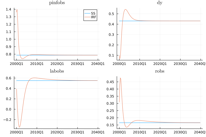
We can now take a look at how some of the observable variables in the model have responded to this shock. We use plot from the Plots package to for that. We specify the variables we want to plot using vars and the names of the datasets being plotted (for the legend) in the names option.
julia> plot(ss, irf,
            trange=sim_rng,
            vars=(:pinfobs, :dy, :labobs, :robs),
            label=["SS" "IRF"],
            legend=[true false false false],
           );
Part 4: Stochastic shocks simulation
Now let's run a simulation with stochastic shocks. We will have random shocks over two years and then have no shocks for several years afterwards to allow time for the economy to return to its steady state.
julia> sim_rng = 2000Q1:2049Q4 # simulate 50 years starting 20002000Q1:2049Q4julia> shk_rng = 2004Q1 .+ (0:7) # shock 8 quarters starting in 20042004Q1:2005Q4julia> p = Plan(m, sim_rng)Plan{MIT{Quarterly{3}}} with range 1999Q2:2050Q1 1999Q2:2050Q1 → ea, eb, eg, em, epinf, eqs, ewjulia> init_rng = first(p.range):first(sim_rng) - 11999Q2:1999Q4julia> final_rng = last(sim_rng) + 1:last(p.range)2050Q1:2050Q1julia> exog = zerodata(m, p);julia> for v in variables(m) exog[init_rng, v] .= m.sstate[v].level end
The distributions of the shocks are assumed normal with mean zero and standard deviations that have been estimated in the replication data. We use packages Distributions and Random to draw the necessary random values.
julia> shk_dist = (ea = Normal(0.0, 0.4618), eb = Normal(0.0, 1.8513), eg = Normal(0.0, 0.6090), eqs = Normal(0.0, 0.6017), em = Normal(0.0, 0.2397), epinf = Normal(0.0, 0.1455), ew = Normal(0.0, 0.2089));julia> for (shk, dist) in pairs(shk_dist) exog[shk_rng, shk] .= rand(dist, length(shk_rng)) endjulia> exog[shk_rng, shocks(m)]8×7 MVTSeries{Quarterly} with range 2004Q1:2005Q4 and variables (ea,eb,eg,…): ea eb … eqs ew 2004Q1 : 0.448249 3.00245 … -0.0873753 0.0245586 2004Q2 : -0.452203 -1.41382 … 1.25253 -0.36206 2004Q3 : 0.416479 -0.989907 … -0.620108 0.0445248 2004Q4 : -0.0151485 -1.54975 … -0.532392 0.140022 2005Q1 : -0.277446 -0.184928 … 1.55412 -0.0826688 2005Q2 : -0.667383 -1.34431 … -0.288241 -0.0395756 2005Q3 : 1.25029 -0.445367 … -0.156082 -0.0248482 2005Q4 : 0.70399 1.74528 … 0.414442 0.283304
Now we are ready to simulate. We can set the shocks to be anticipated or unanticipated by setting the anticipate parameter in simulate.
julia> sim_a = simulate(m, p, exog; fctype=fcslope, anticipate=true);[ Info: Simulating 2000Q1:2049Q4 [ Info: 1, || Fx || = 3.0024525394068884, || Δx || = 25.680188355976632 [ Info: 2, || Fx || = 3.552713678800501e-15julia> sim_u = simulate(m, p, exog; fctype=fcslope, anticipate=false);[ Info: Simulating 2000Q1:2049Q4 with (1.0e-10, 20) [ Info: 1, || Fx || = 0.7869, || Δx || = 0.7869 [ Info: 2, || Fx || = 5.551115123125783e-17 [ Info: Simulating 2004Q1:2049Q4 with (1.0e-10, 20) [ Info: 1, || Fx || = 3.0024525394068884, || Δx || = 27.80863110706991 [ Info: 2, || Fx || = 3.552713678800501e-15 [ Info: Simulating 2004Q2:2049Q4 with (1.0e-10, 20) [ Info: 1, || Fx || = 1.4138173624316919, || Δx || = 15.558219818407464 [ Info: 2, || Fx || = 1.7763568394002505e-15 [ Info: Simulating 2004Q3:2049Q4 with (1.0e-10, 20) [ Info: 1, || Fx || = 0.9899065946591128, || Δx || = 8.41194023914995 [ Info: 2, || Fx || = 1.7763568394002505e-15 [ Info: Simulating 2004Q4:2049Q4 with (1.0e-10, 20) [ Info: 1, || Fx || = 1.5497531321281541, || Δx || = 13.438537019491138 [ Info: 2, || Fx || = 1.7763568394002505e-15 [ Info: Simulating 2005Q1:2049Q4 with (1.0e-10, 20) [ Info: 1, || Fx || = 1.5541237658528908, || Δx || = 11.632044872868242 [ Info: 2, || Fx || = 3.552713678800501e-15 [ Info: Simulating 2005Q2:2049Q4 with (1.0e-10, 20) [ Info: 1, || Fx || = 1.344307287446711, || Δx || = 12.917762840897584 [ Info: 2, || Fx || = 4.440892098500626e-15 [ Info: Simulating 2005Q3:2049Q4 with (1.0e-10, 20) [ Info: 1, || Fx || = 1.2502883762843473, || Δx || = 4.993254894749362 [ Info: 2, || Fx || = 1.1102230246251565e-15 [ Info: Simulating 2005Q4:2049Q4 with (1.0e-10, 20) [ Info: 1, || Fx || = 1.745281307718729, || Δx || = 15.984049604266733 [ Info: 2, || Fx || = 2.1371793224034263e-15 [ Info: Simulating 2005Q4:2049Q4 with (1.0e-10, 20) [ Info: 1, || Fx || = 2.1371793224034263e-15
As before, we can review the responses of the observed variables to these shocks using plot.
julia> observed = (:dy, :dc, :dinve, :labobs, :pinfobs, :dw, :robs);julia> ss = steadystatedata(m, p);julia> plot(ss, sim_a, sim_u, trange=sim_rng, vars=observed, label=["SS", "Anticipated", "Unanticipated"], legend=[true (false for i = 1:6)...], linewidth=1.5, );

We see that when the shocks are anticipated, the variables start to react to them right away; in the unanticipated case, there is no movement until the shocks actually hit.
Part 5: Backing out historical shocks
Now let's pretend that the simulated values are historical data and that we do not know the magnitude of the shocks. We can treat the observed (simulated) values of the variables as known by making them exogenous. At the same time we will make the shocks endogenous, so that we can solve for their values during the simulation.
The "historic" (simulated, assumed observed) range is from the first period of the simulation until the last shock in the previous exercise.
julia> hist_rng = first(sim_rng):last(shk_rng)2000Q1:2005Q4
We use exogenize! and endogenize! to set up a plan in which observed variables are exogenous and shocks are endogenous throughout the historic range.
julia> endogenize!(p, shocks(m), hist_rng);julia> exogenize!(p, observed, hist_rng);julia> pPlan{MIT{Quarterly{3}}} with range 1999Q2:2050Q1 1999Q2:1999Q4 → ea, eb, eg, em, epinf, eqs, ew 2000Q1:2005Q4 → dc, dinve, dw, dy, labobs, pinfobs, robs 2006Q1:2050Q1 → ea, eb, eg, em, epinf, eqs, ew
As we can see above, the plan now reflects our intentions.
Finally, we need to set up the exogenous data. This time we do not specify the shocks; instead, we assign the known data for the observed variables for the historic range. We start with initial conditions.
julia> exog = zerodata(m, p);julia> for v in variables(m) exog[init_rng, v] .= m.sstate[v].level end
We take the observed data from the simulation above. We show the anticipated version first.
julia> for v in observed exog[hist_rng, v] .= sim_a[v] endjulia> back_a = simulate(m, p, exog; fctype=fcslope, anticipate=true);[ Info: Simulating 2000Q1:2049Q4 [ Info: 1, || Fx || = 6.914308327521269, || Δx || = 25.680188355976643 [ Info: 2, || Fx || = 3.552713678800501e-15
Now we show the unanticipated case.
julia> for v in observed exog[hist_rng, v] .= sim_u[v] endjulia> back_u = simulate(m, p, exog; fctype=fcslope, anticipate=false);[ Info: Simulating 2000Q1:2049Q4 with (1.0e-10, 20) [ Info: 1, || Fx || = 6.634422995554733, || Δx || = 6.634422995554732 [ Info: 2, || Fx || = 4.440892098500626e-16 [ Info: Simulating 2004Q1:2049Q4 with (1.0e-10, 20) [ Info: 1, || Fx || = 6.634422995554733, || Δx || = 27.80863110706991 [ Info: 2, || Fx || = 3.552713678800501e-15 [ Info: Simulating 2004Q2:2049Q4 with (1.0e-10, 20) [ Info: 1, || Fx || = 3.1359399254503466, || Δx || = 15.55821981840747 [ Info: 2, || Fx || = 1.7763568394002505e-15 [ Info: Simulating 2004Q3:2049Q4 with (1.0e-10, 20) [ Info: 1, || Fx || = 2.9734383160699633, || Δx || = 8.411940239149951 [ Info: 2, || Fx || = 1.7763568394002505e-15 [ Info: Simulating 2004Q4:2049Q4 with (1.0e-10, 20) [ Info: 1, || Fx || = 4.879241298622106, || Δx || = 13.438537019491129 [ Info: 2, || Fx || = 1.7763568394002505e-15 [ Info: Simulating 2005Q1:2049Q4 with (1.0e-10, 20) [ Info: 1, || Fx || = 6.085766380863383, || Δx || = 11.632044872868233 [ Info: 2, || Fx || = 3.552713678800501e-15 [ Info: Simulating 2005Q2:2049Q4 with (1.0e-10, 20) [ Info: 1, || Fx || = 4.083979758127988, || Δx || = 12.917762840897584 [ Info: 2, || Fx || = 1.7763568394002505e-15 [ Info: Simulating 2005Q3:2049Q4 with (1.0e-10, 20) [ Info: 1, || Fx || = 1.7568941715300272, || Δx || = 4.99325489474936 [ Info: 2, || Fx || = 1.3322676295501878e-15 [ Info: Simulating 2005Q4:2049Q4 with (1.0e-10, 20) [ Info: 1, || Fx || = 4.651463336621746, || Δx || = 15.984049604266735 [ Info: 2, || Fx || = 3.9968028886505635e-15 [ Info: Simulating 2005Q4:2049Q4 with (1.0e-10, 20) [ Info: 1, || Fx || = 3.9968028886505635e-15
If we did everything correctly, the shocks we recovered must match exactly the shocks we used when we simulated the "historical" data.
julia> @test sim_a[shocks(m)] ≈ back_a[shocks(m)]Test Passed Expression: sim_a[shocks(m)] ≈ back_a[shocks(m)] Evaluated: 204×7 MVTSeries{Quarterly} with range 1999Q2:2050Q1 and variables (ea,eb,eg,…): ea eb … eqs ew 1999Q2 : 0.0 0.0 … 0.0 0.0 1999Q3 : 0.0 0.0 … 0.0 0.0 1999Q4 : 0.0 0.0 … 0.0 0.0 2000Q1 : 0.0 0.0 … 0.0 0.0 2000Q2 : 0.0 0.0 … 0.0 0.0 2000Q3 : 0.0 0.0 … 0.0 0.0 2000Q4 : 0.0 0.0 … 0.0 0.0 2001Q1 : 0.0 0.0 … 0.0 0.0 2001Q2 : 0.0 0.0 … 0.0 0.0 ⋮ ⋮ ⋱ ⋮ ⋮ 2048Q1 : 0.0 0.0 … 0.0 0.0 2048Q2 : 0.0 0.0 … 0.0 0.0 2048Q3 : 0.0 0.0 … 0.0 0.0 2048Q4 : 0.0 0.0 … 0.0 0.0 2049Q1 : 0.0 0.0 … 0.0 0.0 2049Q2 : 0.0 0.0 … 0.0 0.0 2049Q3 : 0.0 0.0 … 0.0 0.0 2049Q4 : 0.0 0.0 … 0.0 0.0 2050Q1 : 0.0 0.0 … 0.0 0.0 ≈ 204×7 MVTSeries{Quarterly} with range 1999Q2:2050Q1 and variables (ea,eb,eg,…): ea eb … eqs ew 1999Q2 : 0.0 0.0 … 0.0 0.0 1999Q3 : 0.0 0.0 … 0.0 0.0 1999Q4 : 0.0 0.0 … 0.0 0.0 2000Q1 : -8.18879e-17 5.38914e-18 … 1.16768e-16 5.55112e-17 2000Q2 : 3.98123e-17 -1.33254e-17 … 2.07582e-16 -6.20892e-17 2000Q3 : 7.2593e-17 7.93703e-17 … 7.5955e-17 9.84737e-19 2000Q4 : 1.00073e-16 3.52124e-17 … 2.44976e-17 8.37322e-19 2001Q1 : 6.25075e-17 -4.2643e-17 … 6.71423e-16 -1.1031e-16 2001Q2 : 5.87613e-17 4.77276e-17 … -9.32407e-16 2.73246e-16 ⋮ ⋮ ⋱ ⋮ ⋮ 2048Q1 : 0.0 0.0 … 0.0 0.0 2048Q2 : 0.0 0.0 … 0.0 0.0 2048Q3 : 0.0 0.0 … 0.0 0.0 2048Q4 : 0.0 0.0 … 0.0 0.0 2049Q1 : 0.0 0.0 … 0.0 0.0 2049Q2 : 0.0 0.0 … 0.0 0.0 2049Q3 : 0.0 0.0 … 0.0 0.0 2049Q4 : 0.0 0.0 … 0.0 0.0 2050Q1 : 0.0 0.0 … 0.0 0.0julia> @test sim_u[shocks(m)] ≈ back_u[shocks(m)]Test Passed Expression: sim_u[shocks(m)] ≈ back_u[shocks(m)] Evaluated: 204×7 MVTSeries{Quarterly} with range 1999Q2:2050Q1 and variables (ea,eb,eg,…): ea eb … eqs ew 1999Q2 : 0.0 0.0 … 0.0 0.0 1999Q3 : 0.0 0.0 … 0.0 0.0 1999Q4 : 0.0 0.0 … 0.0 0.0 2000Q1 : 0.0 0.0 … 0.0 0.0 2000Q2 : 0.0 0.0 … 0.0 0.0 2000Q3 : 0.0 0.0 … 0.0 0.0 2000Q4 : 0.0 0.0 … 0.0 0.0 2001Q1 : 0.0 0.0 … 0.0 0.0 2001Q2 : 0.0 0.0 … 0.0 0.0 ⋮ ⋮ ⋱ ⋮ ⋮ 2048Q1 : 0.0 0.0 … 0.0 0.0 2048Q2 : 0.0 0.0 … 0.0 0.0 2048Q3 : 0.0 0.0 … 0.0 0.0 2048Q4 : 0.0 0.0 … 0.0 0.0 2049Q1 : 0.0 0.0 … 0.0 0.0 2049Q2 : 0.0 0.0 … 0.0 0.0 2049Q3 : 0.0 0.0 … 0.0 0.0 2049Q4 : 0.0 0.0 … 0.0 0.0 2050Q1 : 0.0 0.0 … 0.0 0.0 ≈ 204×7 MVTSeries{Quarterly} with range 1999Q2:2050Q1 and variables (ea,eb,eg,…): ea eb … eqs ew 1999Q2 : 0.0 0.0 … 0.0 0.0 1999Q3 : 0.0 0.0 … 0.0 0.0 1999Q4 : 0.0 0.0 … 0.0 0.0 2000Q1 : 0.0 0.0 … 0.0 0.0 2000Q2 : 0.0 0.0 … 0.0 0.0 2000Q3 : 0.0 0.0 … 0.0 0.0 2000Q4 : 0.0 0.0 … 0.0 0.0 2001Q1 : 0.0 0.0 … 0.0 0.0 2001Q2 : 0.0 0.0 … 0.0 0.0 ⋮ ⋮ ⋱ ⋮ ⋮ 2048Q1 : 0.0 0.0 … 0.0 0.0 2048Q2 : 0.0 0.0 … 0.0 0.0 2048Q3 : 0.0 0.0 … 0.0 0.0 2048Q4 : 0.0 0.0 … 0.0 0.0 2049Q1 : 0.0 0.0 … 0.0 0.0 2049Q2 : 0.0 0.0 … 0.0 0.0 2049Q3 : 0.0 0.0 … 0.0 0.0 2049Q4 : 0.0 0.0 … 0.0 0.0 2050Q1 : 0.0 0.0 … 0.0 0.0
Moreover, we must have the unobserved variables match as well. In fact, all the data must match over the entire simulation range.
julia> @test sim_a ≈ back_aTest Passed Expression: sim_a ≈ back_a Evaluated: 204×48 MVTSeries{Quarterly} with range 1999Q2:2050Q1 and variables (a,b,c,cf,…): a b … eqs ew 1999Q2 : 0.0 0.0 … 0.0 0.0 1999Q3 : 0.0 0.0 … 0.0 0.0 1999Q4 : 0.0 0.0 … 0.0 0.0 2000Q1 : 0.0 0.0 … 0.0 0.0 2000Q2 : 0.0 0.0 … 0.0 0.0 2000Q3 : 0.0 0.0 … 0.0 0.0 2000Q4 : 0.0 0.0 … 0.0 0.0 2001Q1 : 0.0 0.0 … 0.0 0.0 2001Q2 : 0.0 0.0 … 0.0 0.0 ⋮ ⋮ ⋱ ⋮ ⋮ 2048Q1 : 0.000908524 7.35776e-112 … 0.0 0.0 2048Q2 : 0.000870094 1.61429e-112 … 0.0 0.0 2048Q3 : 0.000833289 3.54176e-113 … 0.0 0.0 2048Q4 : 0.000798041 7.77062e-114 … 0.0 0.0 2049Q1 : 0.000764283 1.70487e-114 … 0.0 0.0 2049Q2 : 0.000731954 3.74049e-115 … 0.0 0.0 2049Q3 : 0.000700993 8.20664e-116 … 0.0 0.0 2049Q4 : 0.000671341 1.80054e-116 … 0.0 0.0 2050Q1 : 0.000671341 1.80054e-116 … 0.0 0.0 ≈ 204×48 MVTSeries{Quarterly} with range 1999Q2:2050Q1 and variables (a,b,c,cf,…): a b … eqs ew 1999Q2 : 0.0 0.0 … 0.0 0.0 1999Q3 : 0.0 0.0 … 0.0 0.0 1999Q4 : 0.0 0.0 … 0.0 0.0 2000Q1 : -8.18879e-17 5.38914e-18 … 1.16768e-16 5.55112e-17 2000Q2 : -3.86118e-17 -1.21431e-17 … 2.07582e-16 -6.20892e-17 2000Q3 : 3.56144e-17 7.67061e-17 … 7.5955e-17 9.84737e-19 2000Q4 : 1.34181e-16 5.20417e-17 … 2.44976e-17 8.37322e-19 2001Q1 : 1.91013e-16 -3.1225e-17 … 6.71423e-16 -1.1031e-16 2001Q2 : 2.41694e-16 4.08768e-17 … -9.32407e-16 2.73246e-16 ⋮ ⋮ ⋱ ⋮ ⋮ 2048Q1 : 0.000908524 5.05756e-36 … 0.0 0.0 2048Q2 : 0.000870094 1.10937e-36 … 0.0 0.0 2048Q3 : 0.000833289 2.43364e-37 … 0.0 0.0 2048Q4 : 0.000798041 5.34023e-38 … 0.0 0.0 2049Q1 : 0.000764283 1.17205e-38 … 0.0 0.0 2049Q2 : 0.000731954 2.57139e-39 … 0.0 0.0 2049Q3 : 0.000700993 5.64286e-40 … 0.0 0.0 2049Q4 : 0.000671341 1.23852e-40 … 0.0 0.0 2050Q1 : 0.000671341 1.23852e-40 … 0.0 0.0julia> @test sim_u ≈ back_uTest Passed Expression: sim_u ≈ back_u Evaluated: 204×48 MVTSeries{Quarterly} with range 1999Q2:2050Q1 and variables (a,b,c,cf,…): a b … eqs ew 1999Q2 : 0.0 0.0 … 0.0 0.0 1999Q3 : 0.0 0.0 … 0.0 0.0 1999Q4 : 0.0 0.0 … 0.0 0.0 2000Q1 : 0.0 0.0 … 0.0 0.0 2000Q2 : 0.0 0.0 … 0.0 0.0 2000Q3 : 0.0 0.0 … 0.0 0.0 2000Q4 : 0.0 0.0 … 0.0 0.0 2001Q1 : 0.0 0.0 … 0.0 0.0 2001Q2 : 0.0 0.0 … 0.0 0.0 ⋮ ⋮ ⋱ ⋮ ⋮ 2048Q1 : 0.000908524 7.35776e-112 … 0.0 0.0 2048Q2 : 0.000870094 1.61429e-112 … 0.0 0.0 2048Q3 : 0.000833289 3.54176e-113 … 0.0 0.0 2048Q4 : 0.000798041 7.77062e-114 … 0.0 0.0 2049Q1 : 0.000764283 1.70487e-114 … 0.0 0.0 2049Q2 : 0.000731954 3.74049e-115 … 0.0 0.0 2049Q3 : 0.000700993 8.20664e-116 … 0.0 0.0 2049Q4 : 0.000671341 1.80054e-116 … 0.0 0.0 2050Q1 : 0.000671341 1.80054e-116 … 0.0 0.0 ≈ 204×48 MVTSeries{Quarterly} with range 1999Q2:2050Q1 and variables (a,b,c,cf,…): a b … eqs ew 1999Q2 : 0.0 0.0 … 0.0 0.0 1999Q3 : 0.0 0.0 … 0.0 0.0 1999Q4 : 0.0 0.0 … 0.0 0.0 2000Q1 : 0.0 0.0 … 0.0 0.0 2000Q2 : 0.0 0.0 … 0.0 0.0 2000Q3 : 0.0 0.0 … 0.0 0.0 2000Q4 : 0.0 0.0 … 0.0 0.0 2001Q1 : 0.0 0.0 … 0.0 0.0 2001Q2 : 0.0 0.0 … 0.0 0.0 ⋮ ⋮ ⋱ ⋮ ⋮ 2048Q1 : 0.000908524 3.56297e-33 … 0.0 0.0 2048Q2 : 0.000870094 7.82409e-34 … 0.0 0.0 2048Q3 : 0.000833289 1.73033e-34 … 0.0 0.0 2048Q4 : 0.000798041 3.83681e-35 … 0.0 0.0 2049Q1 : 0.000764283 8.36952e-36 … 0.0 0.0 2049Q2 : 0.000731954 1.83377e-36 … 0.0 0.0 2049Q3 : 0.000700993 4.05546e-37 … 0.0 0.0 2049Q4 : 0.000671341 8.96314e-38 … 0.0 0.0 2050Q1 : 0.000671341 8.96314e-38 … 0.0 0.0
Appendix
Replication Data
The replication data can be downloaded from http://doi.org/10.3886/E116269V1